devs <- rnorm(100)
tdevs <- qt(pnorm(devs), df = 1)
plot(devs, tdevs)
abline(0,1)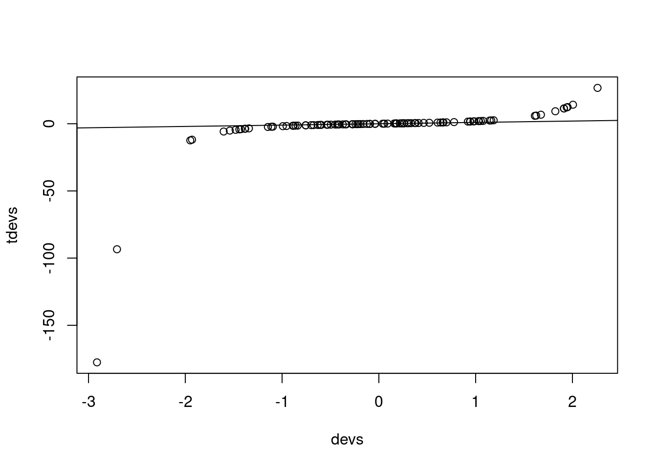
References:
Videos (optional):
There are various videos from 2020 in the bCourses Media Gallery that you can use for reference if you want to.
Many (most?) statistical papers include a simulation (i.e., Monte Carlo) study. Many papers on machine learning methods also include a simulation study. The basic idea is that closed-form mathematical analysis of the properties of a statistical or machine learning method/model is often hard to do. Even if possible, it usually involves approximations or simplifications. A canonical situation in statistics is that we have an asymptotic result and we want to know what happens in finite samples, but often we do not even have the asymptotic result. Instead, we can estimate mathematical expressions using random numbers. So we design a simulation study to evaluate the method/model or compare multiple methods. The result is that the researcher carries out an experiment (on the computer, sometimes called in silico), generally varying different factors to see what has an effect on the outcome of interest.
The basic strategy generally involves simulating data and then using the method(s) on the simulated data, summarizing the results to assess/compare the method(s).
Most simulation studies aim to approximate an integral, generally an expected value (mean, bias, variance, MSE, probability, etc.). In low dimensions, methods such as Gaussian quadrature are best for estimating an integral but these methods don’t scale well (we’ll discuss this in Unit 12 on integration/differentiation), so in higher dimensions we often use Monte Carlo techniques.
To be more concrete:
If we have a method for estimating a model parameter (including uncertainty), such as a regression coefficient, what properties do we want the method to have and what criteria could we use?
If we have a prediction method (including prediction uncertainty), what properties do we want the method to have and what criteria could we use?
If we have a method for doing a hypothesis test, what criteria would we use to assess the hypothesis test? What properties do we want the test to have?
If we have a method for finding a confidence interval or a prediction interval, what criteria would we use to assess the interval?
Let’s consider linear regression, with observations \(Y=(y_{1},y_{2},\ldots,y_{n})\) and an \(n\times p\) matrix of predictors/covariates/features/variables \(X\), where \(\hat{\beta}=(X^{\top}X)^{-1}X^{\top}Y\). If we assume that we have \(EY=X\beta\) and \(\mbox{Var}(Y)=\sigma^{2}I\), then we can determine analytically that we have \[\begin{aligned} E\hat{\beta} & = & \beta\\ \mbox{Var}(\hat{\beta})=E((\hat{\beta}-E\hat{\beta})^{2}) & = & \sigma^{2}(X^{\top}X)^{-1}\\ \mbox{MSPE}(Y^{*})=E(Y^{*}-\hat{Y})^{2}) & = & \sigma^{2}(1+X^{*\top}(X^{\top}X)^{-1}X^{*}).\end{aligned}\] where \(Y^{*}\)is some new observation we’d like to predict given \(X^{*}\).
But suppose that we’re interested in the properties of regression estimation when in reality the mean is not linear in \(X\) or the properties of the errors are more complicated than having independent homoscedastic errors. (This is always the case, but the issue is how far from the truth the standard assumptions are.) Or suppose we have a modified procedure to produce \(\hat{\beta}\), such as a procedure that is robust to outliers. In those cases, we cannot compute the expectations above analytically.
Instead we decide to use a Monte Carlo estimate. To keep the notation more simple, let’s just consider one element of the vector \(\beta\) (i.e., one of the regression coefficients) and continue to call that \(\beta\). If we randomly generate \(m\) different datasets from some distribution \(f\), and \(\hat{\beta}_{i}\) is the estimated coefficient based on the \(i\)th dataset: \(Y_{i}=(y_{i1},y_{i2},\ldots,y_{in})\), then we can estimate \(E\hat{\beta}\) under that distribution \(f\) as
\[\widehat{E(\hat{\beta})}=\bar{\hat{\beta}}=\frac{1}{m}\sum_{i=1}^{m}\hat{\beta}_{i}\]
Or to estimate the variance, we have
\[\widehat{\mbox{Var}(\hat{\beta})}=\frac{1}{m}\sum_{i=1}^{m}(\hat{\beta}_{i}-\bar{\hat{\beta}})^{2}.\]
In evaluating the performance of regression under non-standard conditions or the performance of our robust regression procedure, what decisions do we have to make to be able to carry out our Monte Carlo procedure?
Next let’s think about Monte Carlo methods in general.
The basic idea is that we often want to estimate \(\phi\equiv E_{f}(h(Y))\) for \(Y\sim f\). Note that if \(h\) is an indicator function, this includes estimation of probabilities, e.g., for a scalar \(Y\), we have \(p=P(Y\leq y)=F(y)=\int_{-\infty}^{y}f(t)dt=\int I(t\leq y)f(t)dt=E_{f}(I(Y\leq y))\). We would estimate variances or MSEs by having \(h\) involve squared terms.
We get an MC estimate of \(\phi\) based on an iid sample of a large number of values of \(Y\) from \(f\):
\[\hat{\phi}=\frac{1}{m}\sum_{i=1}^{m}h(Y_{i}),\] which is justified by the Law of Large Numbers:
\[\lim_{m\to\infty}\frac{1}{m}\sum_{i=1}^{m}h(Y_{i})=E_{f}h(Y).\]
Note that in most simulation studies, \(Y\) is an entire dataset (predictors/covariates), and the “iid sample” means generating \(m\) different datasets from \(f\), i.e., \(Y_{i}\in\{Y_{1},\ldots,Y_{m}\}\) not \(m\) different scalar values. If the dataset has \(n\) observations, then \(Y_{i}=(Y_{i1},\ldots,Y_{in})\).
Let’s relate that back to our regression example. In that particular case, if we’re interested in whether the regression estimator is biased, we want to know: \[\phi=E\hat{\beta},\] where \(h(Y) = \hat(\beta)\). We can use the Monte Carlo estimate of \(\phi\):
\[\hat{\phi}=\frac{1}{m}\sum_{i=1}^{m}h(Y_{i})=\frac{1}{m}\sum_{i=1}^{m}\hat{\beta}_{i}=\widehat{E(\hat{\beta})}.\]
For the variance, we have
\[\phi=\mbox{Var}(\hat{\beta})=E_{f}((\hat{\beta}-E\hat{\beta})^{2})\]
and we can use the Monte Carlo estimate of \(\phi\):
\[\hat{\phi}=\frac{1}{m}\sum_{i=1}^{m}h(Y_{i})=\frac{1}{m}\sum_{i=1}^{m}(\hat{\beta}_{i}-E\hat{\beta})^{2}=\widehat{\mbox{Var}(\hat{\beta)}}\]
where \[h(Y)=(\hat{\beta}-E\hat{\beta})^{2}.\]
Finally note that we also need to use the Monte Carlo estimate of \(E\hat{\beta}\) in the Monte Carlo estimation of the variance.
We might also be interested in the coverage of a confidence interval. In that case we have \[h(Y)=1_{\beta\in CI(Y)}\] and we can estimate the coverage as
\[\hat{\phi}=\frac{1}{m}\sum_{i=1}^{m}1_{\beta\in CI(y_{i})}.\]
Of course we want that \(\hat{\phi}\approx1-\alpha\) for a \(100(1-\alpha)\) confidence interval. In the standard case of a 95% interval we want \(\hat{\phi}\approx0.95\).
Since \(\hat{\phi}\) is simply an average of \(m\) identically-distributed values, \(h(Y_{1}),\ldots,h(Y_{m})\), the simulation variance of \(\hat{\phi}\) is \(\mbox{Var}(\hat{\phi})=\sigma^{2}/m\), with \(\sigma^{2}=\mbox{Var}(h(Y))\). An estimator of \(\sigma^{2}=E_{f}((h(Y)-\phi)^{2})\) is \[\begin{aligned} \hat{\sigma}^{2} & = & \frac{1}{m-1}\sum_{i=1}^{m}(h(Y_{i})-\hat{\phi})^{2}\end{aligned}\] So our MC simulation error is based on
\[\widehat{\mbox{Var}}(\hat{\phi})=\frac{\hat{\sigma}^{2}}{m}=\frac{1}{m(m-1)}\sum_{i=1}^{m}(h(Y_{i})-\hat{\phi})^{2}.\]
Note that this is particularly confusing if we have \(\hat{\phi}=\widehat{\mbox{Var}(\hat{\beta})}\) because then we have \(\widehat{\mbox{Var}}(\hat{\phi})=\widehat{\mbox{Var}}(\widehat{\mbox{Var}(\hat{\beta})})\)!
The simulation variance is \(O(\frac{1}{m})\) because we have \(m^{2}\) in the denominator and a sum over \(m\) terms in the numerator.
Note that in the simulation setting, the randomness in the system is very well-defined (as it is in survey sampling, but unlike in most other applications of statistics), because it comes from the RNG that we perform as part of our attempt to estimate \(\phi\). Happily, we are in control of \(m\), so in principle we can reduce the simulation error to as little as we desire. Unhappily, as usual, the standard error goes down with the square root of \(m\).
Some examples of simulation variances we might be interested in in the regression example include:
Uncertainty in our estimate of bias: \(\widehat{\mbox{Var}}(\widehat{E(\hat{\beta})}-\beta)\).
Uncertainty in the estimated variance of the estimated coefficient: \(\widehat{\mbox{Var}}(\widehat{\mbox{Var}(\hat{\beta})})\).
Uncertainty in the estimated mean square prediction error: \(\widehat{\mbox{Var}}(\widehat{\mbox{MSPE}(Y^{*})})\).
In all cases we have to estimate the simulation variance, hence the \(\widehat{\mbox{Var}}()\) notation.
Sometimes the \(Y_{i}\) are generated in a dependent fashion (e.g., sequential MC or MCMC), in which case this variance estimator, \(\widehat{\mbox{Var}}(\hat{\phi})\) does not hold because the samples are not IID, but the estimator \(\hat{\phi}\) is still a valid, unbiased estimator of \(\phi\).
There are some tools for variance reduction in MC settings. One is importance sampling (see Section 3). Others are the use of control variates and antithetic sampling. I haven’t personally run across these latter in practice, so I’m not sure how widely used they are and won’t go into them here.
In some cases we can set up natural strata, for which we know the probability of being in each stratum. Then we would estimate \(\mu\) for each stratum and combine the estimates based on the probabilities. The intuition is that we remove the variability in sampling amongst the strata from our simulation.
Another strategy that comes up in MCMC contexts is Rao-Blackwellization. Suppose we want to know \(E(h(X))\) where \(X=\{X_{1},X_{2}\}\). Iterated expectation tells us that \(E(h(X))=E(E(h(X)|X_{2})\). If we can compute \(E(h(X)|X_{2})=\int h(x_{1},x_{2})f(x_{1}|x_{2})dx_{1}\) then we should avoid introducing stochasticity related to the \(X_{1}\) draw (since we can analytically integrate over that) and only average over stochasticity from the \(X_{2}\) draw by estimating \(E_{X_{2}}(E(h(X)|X_{2})\). The estimator is \[\hat{\mu}_{RB}=\frac{1}{m}\sum_{i=1}^{m}E(h(X)|X_{2,i})\] where we
either draw from the marginal distribution of \(X_{2}\), or equivalently, draw \(X\), but only use \(X_{2}\). Our MC estimator averages over the simulated values of \(X_{2}\). This is called Rao-Blackwellization because it relates to the idea of conditioning on a sufficient statistic. It has lower variance because the variance of each term in the sum of the Rao-Blackwellized estimator is \(\mbox{Var}(E(h(X)|X_{2})\), which is less than the variance in the usual MC estimator, \(\mbox{Var}(h(X))\), based on the usual iterated variance formula: \(V(X)=E(V(X|Y))+V(E(X|Y))\Rightarrow V(E(X|Y))<V(X)\).
Consider the paper that is part of PS5. We can think about designing a simulation study in that context.
First, what are the key issues that need to be assessed to evaluate their methodology?
Second, what do we need to consider in carrying out a simulation study to address those issues? I.e., what are the key decisions to be made in setting up the simulations?
Specify what makes up an individual experiment (i.e., the individual simulated dataset) given a specific set of inputs: sample size, distribution(s) to use, parameter values, statistic of interest, etc. In other words, exactly how would you generate one simulated dataset?
Often you’ll want to see how your results will vary if you change some of the inputs; e.g., sample sizes, parameter values, data generating mechanisms. So determine what factors you’ll want to vary. Each unique combination of input values will be a scenario.
Write code to carry out the individual experiment and return the quantity of interest, with arguments to your code being the inputs that you want to vary.
For each combination of inputs you want to explore (each scenario), repeat the experiment \(m\) times. Note this is an easily parallel calculation (in both the data generating dimension and the inputs dimension(s)).
Summarize the results for each scenario, quantifying simulation uncertainty.
Report the results in graphical or tabular form.
Often a simulation study will compare multiple methods, so you’ll need to do steps 3-6 for each method.
Since a simulation study is an experiment, we should use the same principles of design and analysis we would recommend when advising a practicioner on setting up a scientific experiment.
These include efficiency, reporting of uncertainty, reproducibility and documentation.
In generating the data for a simulation study, we want to think about what structure real data would have that we want to mimic in the simulation study: distributional assumptions, parameter values, dependence structure, outliers, random effects, sample size (\(n\)), etc.
All of these may become input variables in a simulation study. Often we compare two or more statistical methods conditioning on the data context and then assess whether the differences between methods vary with the data context choices. E.g., if we compare an MLE to a robust estimator, which is better under a given set of choices about the data generating mechanism and how sensitive is the comparison to changing the features of the data generating mechanism? So the “treatment variable” is the choice of statistical method. We’re then interested in sensitivity to the conditions (different input values).
Often we can have a large number of replicates (\(m\)) because the simulation is fast on a computer, so we can sometimes reduce the simulation error to essentially zero and thereby avoid reporting uncertainty. To do this, we need to calculate the simulation standard error, generally, \(s/\sqrt{m}\) and see how it compares to the effect sizes. This is particularly important when reporting on the bias of a statistical method.
We might denote the data, which could be the statistical estimator under each of two methods as \(Y_{ijklq}\), where \(q\) indexes treatment, \(j,k,l\) index different additional input variables, and \(i\in\{1,\ldots,m\}\) indexes the replicate. E.g., \(j\) might index whether the data are from a t or normal, \(k\) the value of a parameter, and \(l\) the dataset sample size (i.e., different levels of \(n\)).
One can think about choosing \(m\) based on a basic power calculation, though since we can always generate more replicates, one might just proceed sequentially and stop when the precision of the results is sufficient.
When comparing methods, it’s best to use the same simulated datasets for each level of the treatment variable and to do an analysis that controls for the dataset (i.e., for the random numbers used), thereby removing some variability from the error term. A simple example is to do a paired analysis, where we look at differences between the outcome for two statistical methods, pairing based on the simulated dataset.
One can even use the “same” random number generation for the replicates under different conditions. E.g., in assessing sensitivity to a \(t\) vs. normal data generating mechanism, we might generate the normal RVs and then for the \(t\) use the same random numbers, in the sense of using the same quantiles of the \(t\) as were generated for the normal - this is pretty easy, as seen below. This helps to control for random differences between the datasets.
devs <- rnorm(100)
tdevs <- qt(pnorm(devs), df = 1)
plot(devs, tdevs)
abline(0,1)
A typical context is that one wants to know the effect of multiple input variables on some outcome. Often, scientists, and even statisticians doing simulation studies will vary one input variable at a time. As we know from standard experimental design, this is inefficient.
The standard strategy is to discretize the inputs, each into a small number of levels. If we have a small enough number of inputs and of levels, we can do a full factorial design (potentially with replication). For example if we have three inputs and three levels each, we have \(3^{3}\) different treatment combinations. Choosing the levels in a reasonable way is obviously important.
As the number of inputs and/or levels increases to the point that we can’t carry out the full factorial, a fractional factorial is an option. This carefully chooses which treatment combinations to omit. The goal is to achieve balance across the levels in a way that allows us to estimate lower level effects (in particular main effects) but not all high-order interactions. What happens is that high-order interactions are aliased to (confounded with) lower-order effects. For example you might choose a fractional factorial design so that you can estimate main effects and two-way interactions but not higher-order interactions.
In interpreting the results, I suggest focusing on the decomposition of sums of squares and not on statistical significance. In most cases, we expect the inputs to have at least some effect on the outcome, so the null hypothesis is a straw man. Better to assess the magnitude of the impacts of the different inputs.
When one has a very large number of inputs, one can use the Latin hypercube approach to sample in the input space in a uniform way, spreading the points out so that each input is sampled uniformly. Assume that each input is \(\mathcal{U}(0,1)\) (one can easily transform to whatever marginal distributions you want). Suppose that you can run \(m\) samples. Then for each input variable, we divide the unit interval into \(m\) bins and randomly choose the order of bins and the position within each bin. This is done independently for each variable and then combined to give \(m\) samples from the input space. We would then analyze main effects and perhaps two-way interactions to assess which inputs seem to be most important.
Even amongst statisticians, taking an experimental design approach to a simulation study is not particularly common, but it’s worth considering.
Luke Miratrix (a UCB Stats PhD alum) has prepared a nice tutorial on carrying out a simulation study, including helpful R code. So if the discussion here is not concrete enough or you want to see how to effectively implement such a study, see simulation_tutorial_miratrix.pdf and the similarly named R code file.
Parallel processing is often helpful for simulation studies. The reason is that simulation studies are embarrassingly parallel - we can send each replicate to a different computer processor and then collect the results back, and the speedup should scale directly with the number of processors we used. Since we often need to some sort of looping, writing code in C/C++ and compiling and linking to the code from R may also be a good strategy, albeit one not covered in this course.
Handy functions in R include expand.grid() to get all combinations of a set of vectors and the replicate() function in R, which will carry out the same R expression (often a function call) repeated times. This can replace the use of a for loop with some gains in cleanliness of your code. Storing results in an array is a natural approach.
thetaLevels <- c("low", "med", "hi")
n <- c(10, 100, 1000)
tVsNorm <- c("t", "norm")
levels <- expand.grid(thetaLevels, tVsNorm, n)
## example of replicate() -- generate m sets correlated normals
set.seed(1)
genFun <- function(n, theta = 1){
    u <- rnorm(n)
    x <- runif(n)
    Cov <- exp(-fields::rdist(x)/theta)
    U <- chol(Cov)
    return(cbind(x,crossprod(U, u)))
}
m <- 20
simData <- replicate(m, genFun(100, 1))
dim(simData) # 100 observations by {x, y} values by 20 replicates
[1] 100 2 20Often results are reported simply in tables, but it can be helpful to think through whether a graphical representation is more informative (sometimes it’s not or it’s worse, but in some cases it may be much better). Since you’ll often have a variety of scenarios to display, using trellis plots in ggplot2 via the facet_wrap function will often be a good approach to display how results vary as a function of multiple inputs.
You should set the seed when you start the experiment, so that it’s possible to replicate it. It’s also a good idea to save the current value of the seed whenever you save interim results, so that you can restart simulations (this is particularly helpful for MCMC) at the exact point you left off, including the random number sequence.
To enhance reproducibility, it’s good practice to post your simulation code (and potentially simulated data) on GitHub, on your website, or as supplementary material with the journal. Another person should be able to fully reproduce your results, including the exact random number generation that you did (e.g., you should provide code for how you set the random seed for your randon number generator).
Many journals are requiring increasingly detailed documentation of the code and data used in your work, including code and data for simulations. Here are the American Statistical Association’s requirements on documenting computations in its journals:
“The ASA strongly encourages authors to submit datasets, code, other programs, and/or extended appendices that are directly relevant to their submitted articles. These materials are valuable to users of the ASA’s journals and further the profession’s commitment to reproducible research. Whenever a dataset is used, its source should be fully documented and the data should be made available as on online supplement. Exceptions for reasons of security or confidentiality may be granted by the Editor. Whenever specific code has been used to implement or illustrate the results of a paper, that code should be made available if possible. [.…snip.…] Articles reporting results based on computation should provide enough information so that readers can evaluate the quality of the results. Such information includes estimated accuracy of results, as well as descriptions of pseudorandom-number generators, numerical algorithms, programming languages, and major software components used.”
At the core of simulations is the ability to generate random numbers, and based on that, random variables. On a computer, our goal is to generate sequences of pseudo-random numbers that behave like random numbers but are replicable. The reason that replicability is important is so that we can reproduce the simulation.
Generating a sequence of random standard uniforms is the basis for all generation of random variables, since random uniforms (either a single one or more than one) can be used to generate values from other distributions. Most random numbers on a computer are pseudo-random. The numbers are chosen from a deterministic stream of numbers that behave like random numbers but are actually a finite sequence (recall that both integers and real numbers on a computer are actually discrete and there are finitely many distinct values), so it’s actually possible to get repeats. The seed of a RNG is the place within that sequence where you start to use the pseudo-random numbers.
Many RNG methods are sequential congruential methods. The basic idea is that the next value is \[u_{k}=f(u_{k-1},\ldots,u_{k-j})\mbox{mod}\,m\] for some function, \(f\), and some positive integer \(m\) . Often \(j=1\). mod just means to take the remainder after dividing by \(m\). One then generates the random standard uniform value as \(u_{k}/m\), which by construction is in \([0,1]\).
Given the construction, such sequences are periodic if the subsequence ever reappears, which is of course guaranteed because there is a finite number of possible subsequence values given that all the \(u_{k}\) values are remainders of divisions by a fixed number . One key to a good random number generator (RNG) is to have a very long period.
An example of a sequential congruential method is a basic linear congruential generator: \[u_{k}=(au_{k-1})\mbox{mod}\,m\] with integer \(a\), \(m\), and \(u_{i}\) values. Here the periodicity can’t exceed \(m-1\) (the method is set up so that we never get \(u_{k}=0\) as this causes the algorithm to break), so we only have \(m-1\) possible values. The seed is the initial state, \(u_{0}\) - i.e., the point in the sequence at which we start. By setting the seed you guarantee reproducibility since given a starting value, the sequence is deterministic. In general \(a\) and \(m\) are chosen to be large, but of course they can’t be too large if they are to be represented as computer integers. The standard values of \(m\) are Mersenne primes, which have the form \(2^{p}-1\) (but these are not prime for all \(p\)), with \(m=2^{31}-1\) common. Here’s an example of a linear congruential sampler:
n <- 100
a <- 171
m <- 30269
u <- rep(NA, n)
u[1] <- 7306
for(i in 2:n)
  u[i] <- (a * u[i-1]) %% m
u <- u/m
uFromR <- runif(n)
par(mfrow = c(2,2), mgp = c(1.8, 0.7, 0), mai = c(.5,.5,.3,.1))
plot(1:n, u, type = 'l')
plot(1:n, uFromR, type = 'l')
hist(u, nclass = 25)
hist(uFromR, nclass = 25)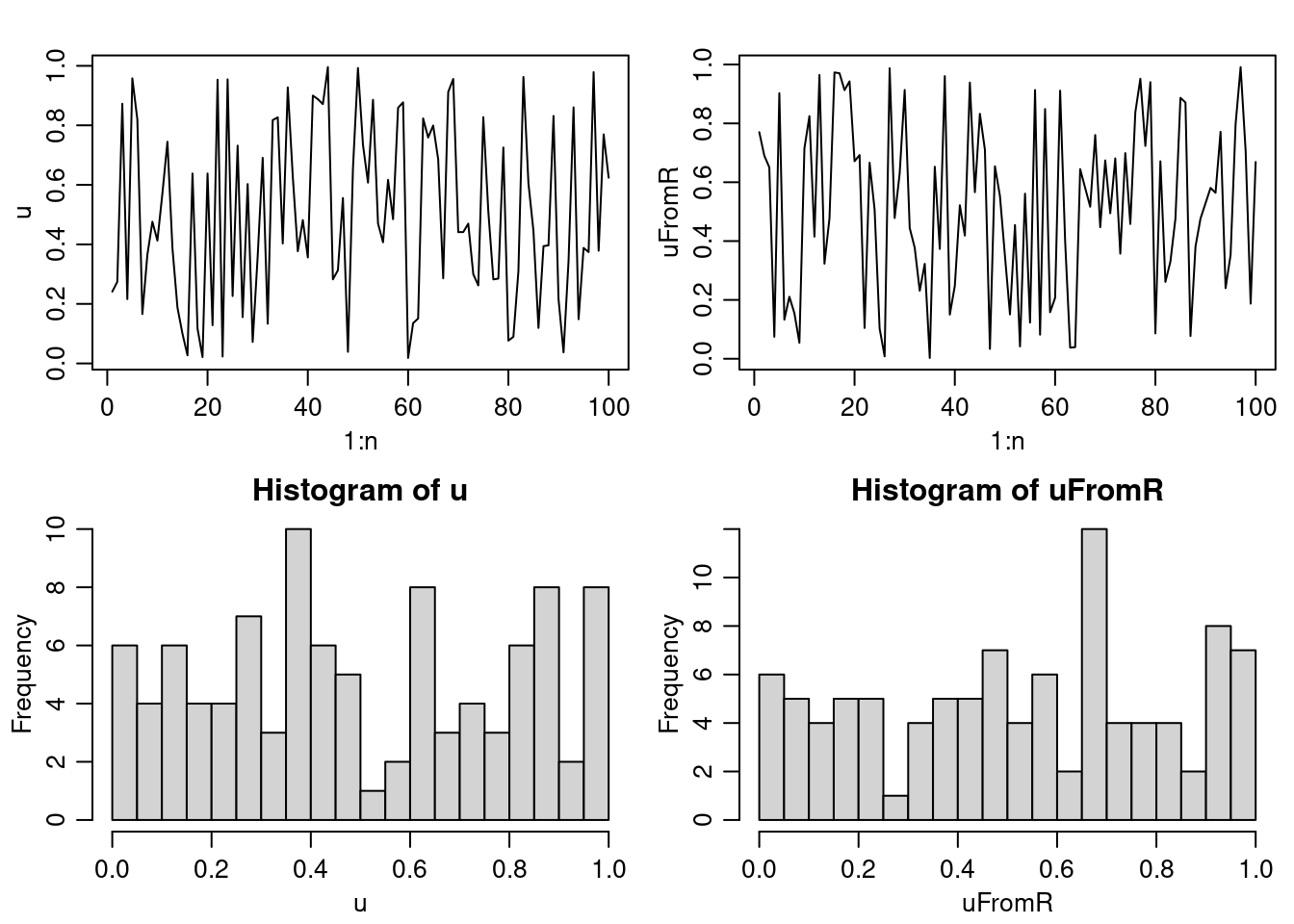
A wide variety of different RNG have been proposed. Many have turned out to have substantial defects based on tests designed to assess if the behavior of the RNG mimics true randomness. Some of the behavior we want to ensure is uniformity of each individual random deviate, independence of sequences of deviates, and multivariate uniformity of subsequences. One test of a RNG that many RNGs don’t perform well on is to assess the properties of \(k\)-tuples - subsequences of length \(k\), which should be independently distributed in the \(k\)-dimensional unit hypercube. Unfortunately, linear congruential methods produce values that lie on a simple lattice in \(k\)-space, i.e., the points are not selected from \(q^{k}\) uniformly spaced points, where \(q\) is the the number of unique values. Instead, points often lie on parallel lines in the hypercube.
Combining generators can yield better generators. The Wichmann-Hill is an option in R and is a combination of three linear congruential generators with \(a=\{171,172,170\}\), \(m=\{30269,30307,30323\}\), and \(u_{i}=(x_{i}/30269+y_{i}/30307+z_{i}/30323)\mbox{mod}\,1\) where \(x\), \(y\), and \(z\) are generated from the three individual generators. Let’s mimic the Wichmann-Hill manually:
RNGkind("Wichmann-Hill")
set.seed(1)
saveSeed <- .Random.seed
uFromR <- runif(10)
a <- c(171, 172, 170)
m <- c(30269, 30307, 30323)
xyz <- matrix(NA, nr = 10, nc = 3)
xyz[1, ] <- (a * saveSeed[2:4]) %% m
for( i in 2:10)
    xyz[i, ] <- (a * xyz[i-1, ]) %% m
for(i in 1:10)
    print(c(uFromR[i],sum(xyz[i, ]/m)%%1))
[1] 0.1297134 0.1297134
[1] 0.9822407 0.9822407
[1] 0.8267184 0.8267184
[1] 0.242355 0.242355
[1] 0.8568853 0.8568853
[1] 0.8408788 0.8408788
[1] 0.3421633 0.3421633
[1] 0.7062672 0.7062672
[1] 0.6212432 0.6212432
[1] 0.6537663 0.6537663## we should be able to recover the current value of the seed
xyz[10, ][1] 24279 14851 10966.Random.seed[2:4][1] 24279 14851 10966By default R uses something called the Mersenne twister, which is in the class of generalized feedback shift registers (GFSR). The basic idea of a GFSR is to come up with a deterministic generator of bits (i.e., a way to generate sequences of 0s and 1s), \(B_{i}\), \(i=1,2,3,\ldots\). The pseudo-random numbers are then determined as sequential subsequences of length \(L\) from \(\{B_{i}\}\), considered as a base-2 number and dividing by \(2^{L}\) to get a number in \((0,1)\). In general the sequence of bits is generated by taking \(B_{i}\) to be the exclusive or [i.e., 0+0 = 0; 0 + 1 = 1; 1 + 0 = 1; 1 + 1 = 0] summation of two previous bits further back in the sequence where the lengths of the lags are carefully chosen.
Generators should give you the same sequence of random numbers, starting at a given seed, whether you ask for a bunch of numbers at once, or sequentially ask for individual numbers.
When one invokes a RNG without a seed, they generally have a method for choosing a seed, often based on the system clock.
There have been some attempts to generate truly random numbers based on physical randomness. One that is based on quantum physics is http://www.idquantique.com/true-random-number-generator/quantis-usb-pcie-pci.html. Another approach is based on lava lamps!
We can change the RNG in R using RNGkind(). We can set the seed with set.seed(). The seed is stored in .Random.seed. The first element indicates the type of RNG (and the type of normal RV generator). The remaining values are specific to the RNG. In the demo code, we’ve seen that for Wichmann-Hill, the remaining three numbers are the current values of \(\{x,y,z\}\).
In R the default RNG is the Mersenne twister (?RNGkind), which is considered to be state-of-the-art – it has some theoretical support, has performed reasonably on standard tests of pseudorandom numbers and has been used without evidence of serious failure. Plus it’s fast (because bitwise operations are fast). In fact this points out one of the nice features of R, which is that for something as important as this, the default is generally carefully chosen by R’s developers. The particular Mersenne twister used has a periodicity of \(2^{19937}-1\approx10^{6000}\). Practically speaking this means that if we generated one random uniform per nanosecond for 10 billion years, then we would generate \(10^{25}\) numbers, well short of the period. So we don’t need to worry about the periodicity! The seed for the Mersenne twister is a set of 624 32-bit integers plus a position in the set, where the position is .Random.seed[2].
We can set the seed by passing an integer to set.seed(), which then sets as many actual seeds as required for a given generator. Here I’ll refer to the integer passed to set.seed() as the seed. Ideally, nearby seeds generally should not correspond to getting sequences from the stream that are closer to each other than far away seeds. According to Gentle (CS, p. 327) the input to set.seed() should be an integer, \(i\in\{0,\ldots,1023\}\) , and each of these 1024 values produces positions in the RNG sequence that are “far away” from each other. I don’t see any mention of this in the R documentation for set.seed() and furthermore, you can pass integers larger than 1023 to set.seed(), so I’m not sure how much to trust Gentle’s claim. More on generating parallel streams of random numbers below.
So we get replicability by setting the seed to a specific value at the beginning of our simulation. We can then set the seed to that same value when we want to replicate the simulation.
set.seed(1)
rnorm(10)
[1] -1.12774688 0.94127649 1.06642978 -0.40656626 0.30874760 1.42146069
[7] -1.68323660 0.43367702 -0.01607178 -1.72752716set.seed(1)
rnorm(10) [1] -1.12774688 0.94127649 1.06642978 -0.40656626 0.30874760 1.42146069
[7] -1.68323660 0.43367702 -0.01607178 -1.72752716We can also save the state of the RNG and pick up where we left off. So this code will pick where you had left off, ignoring what happened in between saving to savedSeed and resetting.
set.seed(1)
rnorm(5)
[1] -1.1277469 0.9412765 1.0664298 -0.4065663 0.3087476savedSeed <- .Random.seed
rnorm(5)[1] 1.42146069 -1.68323660 0.43367702 -0.01607178 -1.72752716tmp <- sample(1:50, 2000, replace = TRUE)
.Random.seed <- savedSeed
rnorm(5)[1] 1.42146069 -1.68323660 0.43367702 -0.01607178 -1.72752716In some cases you might want to reset the seed upon exit from a function so that a user’s random number stream is unaffected:
f <- function(args) {
  oldseed <- .Random.seed
  ## other code
  .Random.seed <<- oldseed # note global assignment!
}
Note the need to reassign to the global variable .Random.seed.
RNGversion() allows you to revert to RNG from previous versions of R, which is very helpful for reproducibility.
The RNGs in R generally return 32-bit (4-byte) integers converted to doubles, so there are at most \(2^{32}\) distinct values. This means you could get duplicated values in long runs, but this does not violate the comment about the periodicity because the two values after the two duplicated numbers will not be duplicates of each other – note there is a distinction between the values as presented to the user and the values as generated by the RNG algorithm.
One way to proceed if you’re using both R and C is to have C use the R RNG, calling the C functions that R uses under the hood, which are located in the Rmath library. This way you have a consistent source of random numbers and don’t need to worry about issues with RNG in C. If you call C from R, this should approach should also work (see details in http://statistics.berkeley.edu/computing/cpp); you could also generate all the random numbers you need in R and pass them to the C function.
Note that whenever a random number is generated, the software needs to retain information about what has been generated, so this is an example where a function must have a side effect not observed by the user. R frowns upon this sort of thing, but it’s necessary in this case.
We can generally rely on the RNG in R to give a reasonable set of values. One time when we want to think harder is when doing work with RNG in parallel on multiple processors. The worst thing that could happen is that one sets things up in such a way that every process is using the same sequence of random numbers. This could happen if you mistakenly set the same seed in each process, e.g., using set.seed(mySeed) in R on every process. More details on parallel RNG are given in Unit 6.
There are a variety of methods for generating from common distributions (normal, gamma, beta, Poisson, t, etc.). Since these tend to be built into R and presumably use good algorithms, we won’t go into them. A variety of statistical computing and Monte Carlo books describe the various methods. Many are built on the relationships between different distributions - e.g., a beta random variable (RV) can be generated from two gamma RVs.
Also note that you can call the C functions that implement the R distribution functions as a library (Rmath), so if you’re coding in C or another language, you should be able to make use of the standard functions: {r,p,q,d}{norm,t,gamma,binom,pois,etc.} (as well as a variety of other R math functions, which can be seen in Rmath.h). Information on this can be found in the Writing R Extensions manual on CRAN (section 6.16).
The mvtnorm package supplies code for working with the density and CDF of multivariate normal and t distributions.
To generate a multivariate normal, in Unit 10, we’ll see the standard method based on the Cholesky decomposition:
U <- chol(covMat)
crossprod(U, rnorm(nrow(covMat)))
Side note: for a singular covariance matrix we can use the Cholesky with pivoting, setting as many rows to zero as the rank deficiency. Then when we generate the multivariate normals, they respect the constraints implicit in the rank deficiency. However, you’ll need to reorder the resulting vector because of the reordering involved in the pivoted Cholesky.
Most of you know the inverse CDF method. To generate \(X\sim F\) where \(F\) is a CDF and is an invertible function, first generate \(Z\sim\mathcal{U}(0,1)\), then \(x=F^{-1}(z)\). For discrete CDFs, one can work with a discretized version. For multivariate distributions, one can work with a univariate marginal and then a sequence of univariate conditionals: \(f(x_{1})f(x_{2}|x_{1})\cdots f(x_{k}|x_{k-1},\ldots,x_{1})\), when the distribution allows this analytic decomposition.
The basic idea of rejection sampling (RS) relies on the introduction of an auxiliary variable, \(u\). Suppose \(X\sim F\). Then we can write \(f(x)=\int_{0}^{f(x)}du\). Thus \(f\) is the marginal density of \(X\) in the joint density, \((X,U)\sim\mathcal{U}\{(x,u):0<u<f(x)\}\). Now we’d like to use this in a way that relies only on evaluating \(f(x)\) without having to draw from \(f\).
To implement this we draw from a larger set and then only keep draws for which \(u<f(x)\). We choose a density, \(g\), that is easy to draw from and that can majorize \(f\), which means there exists a constant \(c\) s.t. , \(cg(x)\geq f(x)\) \(\forall x\). In other words we have that \(cg(x)\) is an upper envelope for \(f(x)\). The algorithm is
The intuition here is graphical: we generate from under a curve that is always above \(f(x)\) and accept only when \(u\) puts us under \(f(x)\) relative to the majorizing density. A key here is that the majorizing density have fatter tails than the density of interest, so that the constant \(c\) can exist. So we could use a \(t\) to generate from a normal but not the reverse. We’d like \(c\) to be small to reduce the number of rejections because it turns out that \(\frac{1}{c}=\frac{\int f(x)dx}{\int cg(x)dx}\) is the acceptance probability. This approach works in principle for multivariate densities but as the dimension increases, the proportion of rejections grows, because more of the volume under \(cg(x)\) is above \(f(x)\).
If \(f\) is costly to evaluate, we can sometimes reduce calculation using a lower bound on \(f\). In this case we accept if \(u\leq f_{\mbox{low}}(y)/cg_{Y}(y)\). If it is not, then we need to evaluate the ratio in the usual rejection sampling algorithm. This is called squeezing.
One example of RS is to sample from a truncated normal. Of course we can just sample from the normal and then reject, but this can be inefficient, particularly if the truncation is far in the tail (a case in which inverse CDF suffers from numerical difficulties). Suppose the truncation point is greater than zero. Working with the standardized version of the normal, you can use an translated exponential with lower end point equal to the truncation point as the majorizing density (Robert 1995; Statistics and Computing, and see calculations in the demo code). For truncation less than zero, just make the values negative.
The difficulty of RS is finding a good enveloping function. Adaptive rejection sampling refines the envelope as the draws occur, in the case of a continuous, differentiable, log-concave density. The basic idea considers the log of the density and involves using tangents or secants to define an upper envelope and secants to define a lower envelope for a set of points in the support of the distribution. The result is that we have piecewise exponentials (since we are exponentiating from straight lines on the log scale) as the bounds. We can sample from the upper envelope based on sampling from a discrete distribution and then the appropriate exponential. The lower envelope is used for squeezing. We add points to the set that defines the envelopes whenever we accept a point that requires us to evaluate \(f(x)\) (the points that are accepted based on squeezing are not added to the set).
Importance sampling (IS) allows us to estimate expected values, with some commonalities with rejection sampling.
\[\phi=E_{f}(h(X))=\int h(x)\frac{f(x)}{g(x)}g(x)dx\] so \(\hat{\phi}=\frac{1}{m}\sum_{i}h(x_{i})\frac{f(x_{i})}{g(x_{i})}\) for \(x_{i}\) drawn from \(g(x)\), where \(w_{i}=f(x_{i})/g(x_{i})\) act as weights. (Often in Bayesian contexts, we know \(f(x)\) only up to a normalizing constant. In this case we need to use \(w_{i}^{*}=w_{i}/\sum_{j}w_{j}\).
Here we don’t require the majorizing property, just that the densities have common support, but things can be badly behaved if we sample from a density with lighter tails than the density of interest. So in general we want \(g\) to have heavier tails. More specifically for a low variance estimator of \(\phi\), we would want that \(f(x_{i})/g(x_{i})\) is large only when \(h(x_{i})\) is very small, to avoid having overly influential points.
This suggests we can reduce variance in an IS context by oversampling \(x\) for which \(h(x)\) is large and undersampling when it is small, since \(\mbox{Var}(\hat{\phi})=\frac{1}{m}\mbox{Var}(h(X)\frac{f(X)}{g(X)})\). An example is that if \(h\) is an indicator function that is 1 only for rare events, we should oversample rare events and then the IS estimator corrects for the oversampling.
What if we actually want a sample from \(f\) as opposed to estimating the expected value above? We can draw \(x\) from the unweighted sample, \(\{x_{i}\}\), with weights \(\{w_{i}\}\). This is called sampling importance resampling (SIR).
If \(U\) and \(V\) are uniform in \(C=\{(u,v):\,0\leq u\leq\sqrt{f(v/u)}\) then \(X=V/U\) has density proportion to \(f\). The basic algorithm is to choose a rectangle that encloses \(C\) and sample until we find \(u\leq f(v/u)\). Then we use \(x=v/u\) as our RV. The larger region enclosing \(C\) is the majorizing region and a simple approach (if \(f(x)\)and \(x^{2}f(x)\) are bounded in \(C\)) is to choose the rectangle, \(0\leq u\leq\sup_{x}\sqrt{f(x)}\), \(\inf_{x}x\sqrt{f(x)}\leq v\leq\sup_{x}x\sqrt{f(x)}\).
One can also consider truncating the rectangular region, depending on the features of \(f\).
Monahan recommends the ratio of uniforms, particularly a version for discrete distributions (p. 323 of the 2nd edition).