import dask
dask.config.set(scheduler='threads', num_workers = 4)
import dask.dataframe as ddf
path = '/scratch/users/paciorek/243/AirlineData/csvs/'
air = ddf.read_csv(path + '*.csv.bz2',
      compression = 'bz2',
      encoding = 'latin1', # (unexpected) latin1 value(s) in TailNum field in 2001
      dtype = {'Distance': 'float64', 'CRSElapsedTime': 'float64',
      'TailNum': 'object', 'CancellationCode': 'object'})
# specify dtypes so Pandas doesn't complain about column type heterogeneity
airBig data and databases
References:
- Tutorial on parallel processing using Python’s Dask and R’s future packages
- Tutorial on working with large datasets in SQL, R, and Python
- Murrell: Introduction to Data Technologies
- Adler: R in a Nutshell
- Spark Programming Guide
I’ve also pulled material from a variety of other sources, some mentioned in context below.
Note that for a lot of the demo code I ran the code separately from rendering this document because of the time involved in working with large datasets.
We’ll focus on Dask and databases/SQL in this Unit. The material on using Spark is provided for reference, but you’re not responsible for that material. If you’re interested in working with big datasets in R or with tools other than Dask in Python, there is some material in the tutorial on working with large datasets.
Videos:
As posted in the Discussion Forum, please review the five videos on databases and SQL to accompany Section 3 of this Unit. Note that I recorded these videos in fall 2020, so there are occasional references to Unit 8, rather than Unit 7 because I’ve reordered the units of the class a bit since 2020.
- Video 1. Database schema and normalization
- Video 2. Stack Overflow database example
- Video 3. Basic SQL queries
- Video 4. Database joins
- Video 5. Database indxes
1. A few preparatory notes
An editorial on ‘big data’
‘Big data’ is trendy these days, though I guess it’s not quite the buzzword/buzzphrase that it was a few years ago.
Personally, I think some of the hype is justified and some is hype. Large datasets allow us to address questions that we can’t with smaller datasets, and they allow us to consider more sophisticated (e.g., nonlinear) relationships than we might with a small dataset. But they do not directly help with the problem of correlation not being causation. Having medical data on every American still doesn’t tell me if higher salt intake causes hypertension. Internet transaction data does not tell me if one website feature causes increased viewership or sales. One either needs to carry out a designed experiment or think carefully about how to infer causation from observational data. Nor does big data help with the problem that an ad hoc ‘sample’ is not a statistical sample and does not provide the ability to directly infer properties of a population. Consider the immense difficulties we’ve seen in answering questions about Covid despite large amounts of data, because it is incomplete/non-representative. A well-chosen smaller dataset may be much more informative than a much larger, more ad hoc dataset. However, having big datasets might allow you to select from the dataset in a way that helps get at causation or in a way that allows you to construct a population-representative sample. Finally, having a big dataset also allows you to do a large number of statistical analyses and tests, so multiple testing is a big issue. With enough analyses, something will look interesting just by chance in the noise of the data, even if there is no underlying reality to it.
Different people define the ‘big’ in big data differently. One definition involves the actual size of the data, and in some cases the speed with which it is collected. Our efforts here will focus on dataset sizes that are large for traditional statistical work but would probably not be thought of as large in some contexts such as Google or the US National Security Agency (NSA). Another definition of ‘big data’ has more to do with how pervasive data and empirical analyses backed by data are in society and not necessarily how large the actual dataset size is.
Logistics and data size
One of the main drawbacks with R (and Python) in working with big data is that all objects are stored in memory, so you can’t directly work with datasets that are more than 1-20 Gb or so, depending on the memory on your machine.
The techniques and tools discussed in this Unit (apart from the section on MapReduce/Spark) are designed for datasets in the range of gigabytes to tens of gigabytes, though they may scale to larger if you have a machine with a lot of memory or simply have enough disk space and are willing to wait. If you have 10s of gigabytes of data, you’ll be better off if your machine has 10s of GBs of memory, as discussed in this Unit.
If you’re scaling to 100s of GBs, terabytes or petabytes, tools such as carefully-administered databases, cloud-based tools such as provided by AWS and Google Cloud Platform, and Spark or other such tools are probably your best bet.
Note: in handling big data files, it’s best to have the data on the local disk of the machine you are using to reduce traffic and delays from moving data over the network.
What we already know about handling big data!
UNIX operations are generally very fast, so if you can manipulate your data via UNIX commands and piping, that will allow you to do a lot. We’ve already seen UNIX commands for extracting columns. And various commands such as grep, head, tail, etc. allow you to pick out rows based on certain criteria. As some of you have done in problem sets, one can use awk to extract rows. So basic shell scripting may allow you to reduce your data to a more manageable size.
The tool GNU parallel allows you to parallelize operations from the command line and is commonly used in working on Linux clusters.
And don’t forget simple things. If you have a dataset with 30 columns that takes up 10 Gb but you only need 5 of the columns, get rid of the rest and work with the smaller dataset. Or you might be able to get the same information from a random sample of your large dataset as you would from doing the analysis on the full dataset. Strategies like this will often allow you to stick with the tools you already know.
Also, remember that we can often store data more compactly in binary formats than in flat text (e.g., csv) files.
Finally, for many applications, storing large datasets in a standard database will work well.
2. MapReduce, Dask, Hadoop, and Spark
Traditionally, high-performance computing (HPC) has concentrated on techniques and tools for message passing such as MPI and on developing efficient algorithms to use these techniques. In the last 20 years, focus has shifted to technologies for processing large datasets that are distributed across multiple machines but can be manipulated as if they are one dataset.
Two commonly-used tools for doing this are Spark and Python’s Dask package. We’ll cover Dask.
Overview
A basic paradigm for working with big datasets is the MapReduce paradigm. The basic idea is to store the data in a distributed fashion across multiple nodes and try to do the computation in pieces on the data on each node. Results can also be stored in a distributed fashion.
A key benefit of this is that if you can’t fit your dataset on disk on one machine you can on a cluster of machines. And your processing of the dataset can happen in parallel. This is the basic idea of MapReduce.
The basic steps of MapReduce are as follows:
- read individual data objects (e.g., records/lines from CSVs or individual data files)
- map: create key-value pairs using the inputs (more formally, the map step takes a key-value pair and returns a new key-value pair)
- reduce: for each key, do an operation on the associated values and create a result - i.e., aggregate within the values assigned to each key
- write out the {key,result} pair
A similar paradigm that is implemented in dplyr is the split-apply-combine strategy, discussed a bit in Unit 5.
A few additional comments. In our map function, we could exclude values or transform them in some way, including producing multiple records from a single record. And in our reduce function, we can do more complicated analysis. So one can actually do fairly sophisticated things within what may seem like a restrictive paradigm. But we are constrained such that in the map step, each record needs to be treated independently and in the reduce step each key needs to be treated independently. This allows for the parallelization.
One important note is that any operations that require moving a lot of data between the workers can take a long time. (This is sometimes called a shuffle.) This could happen if, for example, you computed the median value within each of many groups if the data for each group are spread across the workers. In contrast, if we compute the mean or sum, one can compute the partial sums on each worker and then just add up the partial sums.
Note that as discussed in Unit 5 the concepts of map and reduce are core concepts in functional programming, and the various apply and lapply style commands are base R’s version of a map operation.
Hadoop is an infrastructure for enabling MapReduce across a network of machines. The basic idea is to hide the complexity of distributing the calculations and collecting results. Hadoop includes a file system for distributed storage (HDFS), where each piece of information is stored redundantly (on multiple machines). Calculations can then be done in a parallel fashion, often on data in place on each machine thereby limiting the amount of communication that has to be done over the network. Hadoop also monitors completion of tasks and if a node fails, it will redo the relevant tasks on another node. Hadoop is based on Java. Given the popularity of Spark, I’m not sure how much usage these approaches currently see. Setting up a Hadoop cluster can be tricky. Hopefully if you’re in a position to need to use Hadoop, it will be set up for you and you will be interacting with it as a user/data analyst.
Ok, so what is Spark? You can think of Spark as in-memory Hadoop. Spark allows one to treat the memory across multiple nodes as a big pool of memory. Therefore, Spark should be faster than Hadoop when the data will fit in the collective memory of multiple nodes. In cases where it does not, Spark will make use of the HDFS (and generally, Spark will be reading the data initially from HDFS.) While Spark is more user-friendly than Hadoop, there are also some things that can make it hard to use. Setting up a Spark cluster also involves a bit of work, Spark can be hard to configure for optimal performance, and Spark calculations have a tendency to fail (often involving memory issues) in ways that are hard for users to debug.
Using Dask for big data processing
Unit 6 on parallelization gives an overview of using Dask in similar fashion to how we used R’s future package for flexible parallelization on different kinds of computational resources (in particular, parallelizing across multiple cores on one machine versus parallelizing across multiple cores across multiple machines/ndoes).
Here we’ll see the use of Dask to work with distributed datasets. Dask can process datasets (potentially very large ones) by parallelizing operations across subsets of the data using multiple cores on one or more machines.
Like Spark, Dask automatically reads data from files in parallel and operates on chunks (also called partitions or shards) of the full dataset in parallel. There are two big advantages of this:
- You can do calculations (including reading from disk) in parallel because each worker will work on a piece of the data.
- When the data is split across machines, you can use the memory of multiple machines to handle much larger datasets than would be possible in memory on one machine. That said, Dask processes the data in chunks, so one often doesn’t need a lot of memory, even just on one machine.
While reading from disk in parallel is a good goal, if all the data are on one hard drive, there are limitations on the speed of reading the data from disk because of having multiple processes all trying to access the disk at once. Supercomputing systems will generally have parallel file systems that support truly parallel reading (and writing, i.e., parallel I/O). Hadoop/Spark deal with this by distributing across multiple disks, generally one disk per machine/node.
Because computations are done in external compiled code (e.g., via numpy) it’s effective to use the threads scheduler when operating on one node to avoid having to copy and move the data.
Dask dataframes (pandas)
Dask dataframes are Pandas-like dataframes where each dataframe is split into groups of rows, stored as smaller Pandas dataframes.
One can do a lot of the kinds of computations that you would do on a Pandas dataframe on a Dask dataframe, but many operations are not possible. See here.
By default dataframes are handled by the threads scheduler. (Recall we discussed Dask’s various schedulers in Unit 6.)
Here’s an example of reading from a dataset of flight delays (about 11 GB data). You can get the data here.
Dask will reads the data in parallel from the various .csv.bz2 files (unzipping on the fly), but note the caveat in the previous section about the possibilities for truly parallel I/O.
However, recall that Dask uses delayed evaluation. In this case, the reading is delayed until compute() is called. For that matter, the various other calculations (max, groupby, mean) shown below are only done after compute() is called.
air.DepDelay.max().compute()   # this takes a while
sub = air[(air.UniqueCarrier == 'UA') & (air.Origin == 'SFO')]
byDest = sub.groupby('Dest').DepDelay.mean()
byDest.compute()               # this takes a while too
You should see this:
    Dest
    ACV 26.200000
    BFL 1.000000
    BOI 12.855069
    BOS 9.316795
    CLE 4.000000
    ...
Note: calling compute twice is a bad idea as Dask will read in the data twice - more on this in a bit.
Dask bags
Bags are like lists but there is no particular ordering, so it doesn’t make sense to ask for the i’th element.
You can think of operations on Dask bags as being like parallel map operations on lists in Python or R.
By default bags are handled via the multiprocessing scheduler.
Let’s see some basic operations on a large dataset of Wikipedia log files. You can get a subset of the Wikipedia data here.
Here we again read the data in (which Dask will do in parallel):
import dask.multiprocessing
dask.config.set(scheduler='processes', num_workers = 4)
import dask.bag as db
## This is the full data
## path = '/scratch/users/paciorek/wikistats/dated_2017/'
## For demo we'll just use a small subset
path = '/scratch/users/paciorek/wikistats/dated_2017_small/dated/'
wiki = db.read_text(path + 'part-0000*gz')
Here we’ll just count the number of records.
import time
t0 = time.time()
wiki.count().compute()
time.time() - t0   # 136 sec. for full data
And here is a more realistic example of filtering (subsetting).
import re
def find(line, regex = 'Armenia'):
    vals = line.split(' ')
    if len(vals) < 6:
        return(False)
    tmp = re.search(regex, vals[3])
    if tmp is None:
        return(False)
    else:
        return(True)


wiki.filter(find).count().compute()
armenia = wiki.filter(find)
smp = armenia.take(100) ## grab a handful as proof of concept
smp[0:5]
Note that it is quite inefficient to do the find() (and implicitly reading the data in) and then compute on top of that intermediate result in two separate calls to compute(). Rather, we should set up the code so that all the operations are set up before a single call to compute(). More on this the Dask/future tutorial
Since the data are just treated as raw strings, we might want to introduce structure by converting each line to a tuple and then converting to a data frame.
def make_tuple(line):
    return(tuple(line.split(' ')))

dtypes = {'date': 'object', 'time': 'object', 'language': 'object',
'webpage': 'object', 'hits': 'float64', 'size': 'float64'}

## Let's create a Dask dataframe.
## This will take a while if done on full data.
df = armenia.map(make_tuple).to_dataframe(dtypes)
type(df)

## Now let's actually do the computation, returning a Pandas df
result = df.compute()
type(result)
result.head()
Dask arrays (numpy)
Dask arrays are numpy-like arrays where each array is split up by both rows and columns into smaller numpy arrays.
One can do a lot of the kinds of computations that you would do on a numpy array on a Dask array, but many operations are not possible. See here.
By default arrays are handled via the threads scheduler.
Non-distributed arrays
Let’s first see operations on a single node, using a single 13 GB two-dimensional array. Again, Dask uses lazy evaluation, so creation of the array doesn’t happen until an operation requiring output is done.
import dask
dask.config.set(scheduler = 'threads', num_workers = 4)
import dask.array as da
x = da.random.normal(0, 1, size=(40000,40000), chunks=(10000, 10000))
# square 10k x 10k chunks
mycalc = da.mean(x, axis = 1)  # by row
import time
t0 = time.time()
rs = mycalc.compute()
time.time() - t0  # 41 sec.
For a row-based operation, we would presumably only want to chunk things up by row, but this doesn’t seem to actually make a difference, presumably because the mean calculation can be done in pieces and only a small number of summary statistics moved between workers.
import dask
dask.config.set(scheduler='threads', num_workers = 4)
import dask.array as da
# x = da.from_array(x, chunks=(2500, 40000))  # adjust chunk size of existing array
x = da.random.normal(0, 1, size=(40000,40000), chunks=(2500, 40000))
mycalc = da.mean(x, axis = 1)  # row means
import time
t0 = time.time()
rs = mycalc.compute()
time.time() - t0   # 42 sec.
Of course, given the lazy evaluation, this timing comparison is not just timing the actual row mean calculations.
But this doesn’t really clarify the story…
import dask
dask.config.set(scheduler='threads', num_workers = 4)
import dask.array as da
import numpy as np
import time
t0 = time.time()
x = np.random.normal(0, 1, size=(40000,40000))
time.time() - t0   # 110 sec.
# for some reason the from_array and da.mean calculations are not done lazily here
t0 = time.time()
dx = da.from_array(x, chunks=(2500, 40000))
time.time() - t0   # 27 sec.
t0 = time.time()
mycalc = da.mean(x, axis = 1)  # what is this doing given .compute() also takes time?
time.time() - t0   # 28 sec.
t0 = time.time()
rs = mycalc.compute()
time.time() - t0   # 21 sec.
Dask will avoid storing all the chunks in memory. (It appears to just generate them on the fly.) Here we have an 80 GB array but we never use more than a few GB of memory (based on top or free -h).
import dask
dask.config.set(scheduler='threads', num_workers = 4)
import dask.array as da
x = da.random.normal(0, 1, size=(100000,100000), chunks=(10000, 10000))
mycalc = da.mean(x, axis = 1)  # row means
import time
t0 = time.time()
rs = mycalc.compute()
time.time() - t0   # 205 sec.
rs[0:5]
Distributed arrays
Using arrays distributed across multiple machines should be straightforward based on using Dask distributed. However, one would want to be careful about creating arrays by distributing the data from a single Python process as that would involve copying between machines.
Spark (optional)
Note for 2019-2022: in past years we covered the use of Spark for processing big datasets. This year we’ll cover similar functionality in Python’s Dask package. I’ve kept this section (and related code in the code files) in case anyone is interested in learning more about Spark, but we won’t cover it in class this year.
Overview
We’ll focus on Spark rather than Hadoop for the speed reasons described above and because I think Spark provides a nicer environment/interface in which to work. Plus it comes out of the (former) AmpLab here at Berkeley. We’ll start with the Python interface to Spark and then see a bit of the sparklyr R package for interfacing with Spark.
More details on Spark are in the Spark programming guide.
Some key aspects of Spark:
- Spark can read/write from various locations, but a standard location is the HDFS, with read/write done in parallel across the cores of the Spark cluster.
- The basic data structure in Spark is a Resilient Distributed Dataset (RDD), which is basically a distributed dataset of individual units, often individual rows loaded from text files.
- RDDs are stored in chunks called partitions, stored on the different nodes of the cluster (either in memory or if necessary on disk).
- Spark has a core set of methods that can be applied to RDDs to do operations such as filtering/subsetting, transformation/mapping, reduction, and others.
- The operations are done in parallel on the different partitions of the data
- Some operations such as reduction generally involve a shuffle, moving data between nodes of the cluster. This is costly.
- Recent versions of Spark have a distributed DataFrame data structure and the ability to run SQL queries on the data.
Question: what do you think are the tradeoffs involved in determining the number of partitions to use?
Note that some headaches with Spark include:
- whether and how to set the amount of memory available for Spark workers (executor memory) and the Spark master process (driver memory)
- hard-to-diagnose failures (including out-of-memory issues)
Getting started
We’ll use Spark on Savio. You can also use Spark on NSF’s XSEDE Bridges supercomputer (among other XSEDE resources), and via commercial cloud computing providers, as well as on your laptop (but obviously only to experiment with small datasets). The demo works with a dataset of Wikipedia traffic, ~110 GB of zipped data (~500 GB unzipped) from October-December 2008, though for in-class presentation we’ll work with a much smaller set of 1 day of data.
The Wikipedia traffic are available through Amazon Web Services storage. The steps to get it are:
- Start an AWS EC2 virtual machine that mounts the data onto the VM
- Install Globus on the VM
- Transfer the data to Savio via Globus
Details on how I did this are in get_wikipedia_data.sh. The resulting data are available to you in /global/scratch/paciorek/wikistats_full/raw on Savio.
Storing data for use in Spark
In many Spark contexts, the data would be stored in a distributed fashion across the hard drives attached to different nodes of a cluster (i.e., in the HDFS).
On Savio, Spark is set up to just use the scratch file system, so one would NOT run the code here, but I’m including it to give a sense for what it’s like to work with HDFS. First we would need to get the data from the standard filesystem to the HDFS. Note that the file system commands are like standard UNIX commands, but you need to do hadoop fs in front of the command.
## DO NOT RUN THIS CODE ON SAVIO ##
## data for Spark on Savio is stored in scratch ##

hadoop fs -ls /
hadoop fs -ls /user
hadoop fs -mkdir /user/paciorek/data
hadoop fs -mkdir /user/paciorek/data/wikistats
hadoop fs -mkdir /user/paciorek/data/wikistats/raw
hadoop fs -mkdir /user/paciorek/data/wikistats/dated

hadoop fs -copyFromLocal /global/scratch/paciorek/wikistats/raw/* \
       /user/paciorek/data/wikistats/raw

# check files on the HDFS, e.g.:
hadoop fs -ls /user/paciorek/data/wikistats/raw

## now do some processing with Spark, e.g., preprocess.{sh,py}

# after processing can retrieve data from HDFS as needed
hadoop fs -copyToLocal /user/paciorek/data/wikistats/dated .
Using Spark on Savio
Here are the steps to use Spark on Savio. We’ll demo using an interactive job (the srun line here) but one could include the last three commands in the SLURM job script.
tmux new -s spark  ## to get back in if disconnected: tmux a -t spark

## having some trouble with ic_stat243 and 4 nodes; check again
srun -A ic_stat243 -p savio2 --nodes=4 -t 1:00:00 --pty bash
module load java spark/2.1.0 python/3.5
source /global/home/groups/allhands/bin/spark_helper.sh
spark-start
## note the environment variables created
env | grep SPARK

spark-submit --master $SPARK_URL  $SPARK_DIR/examples/src/main/python/pi.py
First we’ll load Python; then we can use Spark via the Python interface interactively. We’ll see how to submit batch jobs later.
pyspark --master $SPARK_URL --conf "spark.executorEnv.PYTHONHASHSEED=321" --executor-memory 60G Preprocessing the Wikipedia traffic data
At this point, one complication is that the date-time information on the Wikipedia traffic is embedded in the file names. We’d like that information to be fields in the data files. This is done by running the code in preprocess_wikipedia.py in the Python interface to Spark (pyspark). Note that trying to use multiple nodes and to repartition in various ways caused various errors I was unable to diagnose, but the code as is should work albeit somewhat slowly.
In principle one could run preprocess_wikipedia.py as a batch submission, but I was having problems getting that to run successfully.
Spark in action: processing the Wikipedia traffic data
Now we’ll do some basic manipulations with the Wikipedia dataset, with the goal of analyzing traffic to Barack Obama’s sites during the time around his election as president in 2008. Here are the steps we’ll follow:
- Count the number of lines/observations in our dataset.
- Filter to get only the Barack Obama sites.
- Map step that creates key-value pairs from each record/observation/row.
- Reduce step that counts the number of views by hour and language, so hour-day-lang will serve as the key.
- Map step to prepare the data so it can be output in a nice format.
Note that Spark uses lazy evaluation. Actual computation only happens when one asks for a result to be returned or output written to disk.
First we’ll see how we read in the data and filter to the observations (lines / rows) of interest.
dir = '/global/scratch/paciorek/wikistats'

### read data and do some checks ###

## 'sc' is the SparkContext management object, created via PySpark
## if you simply start Python, without invoking PySpark,
## you would need to create the SparkContext object yourself

lines = sc.textFile(dir + '/' + 'dated')

lines.getNumPartitions()  # 16800 (480 input files) for full dataset

# note delayed evaluation
lines.count()  # 9467817626 for full dataset

# watch the UI and watch wwall as computation progresses

testLines = lines.take(10)
testLines[0]
testLines[9]

### filter to sites of interest ###

import re
from operator import add

def find(line, regex = "Barack_Obama", language = None):
    vals = line.split(' ')
    if len(vals) < 6:
        return(False)
    tmp = re.search(regex, vals[3])
    if tmp is None or (language != None and vals[2] != language):
        return(False)
    else:
        return(True)

lines.filter(find).take(100) # pretty quick

# not clear if should repartition; will likely have small partitions if not
# obama = lines.filter(find).repartition(480) # ~ 18 minutes for full dataset (but remember lazy evaluation)
obama = lines.filter(find)  # use this for demo in section
obama.count()  # 433k observations for full dataset
Now let’s use the mapReduce paradigm to get the aggregate statistics we want.
### map-reduce step to sum hits across date-time-language triplets ###

def stratify(line):
    # create key-value pairs where:
    #   key = date-time-language
    #   value = number of website hits
    vals = line.split(' ')
    return(vals[0] + '-' + vals[1] + '-' + vals[2], int(vals[4]))

# sum number of hits for each date-time-language value
counts = obama.map(stratify).reduceByKey(add)  # 5 minutes
# 128889 for full dataset

### map step to prepare output ###

def transform(vals):
    # split key info back into separate fields
    key = vals[0].split('-')
    return(",".join((key[0], key[1], key[2], str(vals[1]))))

### output to file ###

# have one partition because one file per partition is written out
outputDir = dir + '/' + 'obama-counts'
counts.map(transform).repartition(1).saveAsTextFile(outputDir) # 5 sec.
Spark monitoring
There are various interfaces to monitor Spark and the HDFS.
http://<master_url>:8080general information about the Spark clusterhttp://<master_url>:4040information about the Spark tasks being executedhttp://<master_url>:50070information about the HDFS
When one runs spark-start on Savio, it mentions some log files. If you look in the log file for the master, you should see a line that says “Bound MasterWebUI to 0.0.0.0 and started at http://10.0.5.93:8080” that indicates what the <master_url> is (here it is 10.0.5.93). We need to connect to that URL to view the web UI.
Spark operations
Let’s consider some of the core methods we used.
filter: create a subsetmap: take an RDD and apply a function to each element, returning an RDDreduceandreduceByKey: take an RDD and apply a reduction operation to the elements, doing the reduction stratified by the key values forreduceByKey. Reduction functions need to be associative (order across records doesn’t matter) and commutative (order of arguments doesn’t matter) and take 2 arguments and return 1, all so that they can be done in parallel in a straightforward way.collect: collect results back to the mastercache: tell Spark to keep the RDD in memory for later userepartition: rework the RDD so it is divided into the specified number of partitions
Note that all of the various operations are OOP methods applied to either the SparkContext management object or to a Spark dataset, called a Resilient Distributed Dataset (RDD). Here lines, obama, and counts are all RDDs. However the result of collect() is just a standard Python object.
Nonstandard reduction
Finding the median of a set of values is an example where we don’t have a simple commutative/associative reducer function. Instead we group all the observations for each key into a so-called iterable object. Then our second map function treats each key as an element, iterating over the observations grouped within each key.
As an example we could find the median page size by language (this is not a particularly interesting/useful computation in this dataset, but I wanted to illustrate how this would work).
import numpy as np

def findShortLines(line):
    vals = line.split(' ')
    if len(vals) < 6:
        return(False)
    else:
        return(True)


def computeKeyValue(line):
    vals = line.split(' ')
    # key is language, val is page size
    return(vals[2], int(vals[5]))


def medianFun(input):
    # input[1] is an iterable object containing the page sizes for one key
    # this list comprehension syntax creates a list from the iterable object
    med = np.median([val for val in input[1]])
    # input[0] is the key
    # return a tuple of the key and the median for that key
    return((input[0], med))


output = lines.filter(findShortLines).map(computeKeyValue).groupByKey()
medianResults = output.map(medianFun).collect()
Note that because we need to aggregate all the data by key before doing the reduction on the full data in each key (which is actually just a map operation in this case once the data are already grouped by key), this is much slower than a reduce operation like max or mean.
Spark DataFrames and SQL queries
In recent versions of Spark, one can work with more structured data objects than RDDs. Spark now provides DataFrames, which are collections of row and behave like distributed versions of R or Pandas dataframes. DataFrames seem to be taking the place of RDDs, at least for general, high-level use. They can also be queried using SQL syntax.
Here’s some example code for using DataFrames.
dir = '/global/scratch/paciorek/wikistats'

lines = sc.textFile(dir + '/' + 'dated')

### create DataFrame and do some operations on it ###

def remove_partial_lines(line):
    vals = line.split(' ')
    if len(vals) < 6:
        return(False)
    else:
        return(True)

def create_df_row(line):
    p = line.split(' ')
    return(int(p[0]), int(p[1]), p[2], p[3], int(p[4]), int(p[5]))


tmp = lines.filter(remove_partial_lines).map(create_df_row)

## 'sqlContext' is the Spark sqlContext management object, created via PySpark
## if you simply start Python without invoking PySpark,
## you would need to create the sqlContext object yourself

df = sqlContext.createDataFrame(tmp, schema = ["date", "hour", "lang", "site", "hits", "size"])

df.printSchema()

## note similarity to dplyr and R/Pandas dataframes
df.select('site').show()
df.filter(df['lang'] == 'en').show()
df.groupBy('lang').count().show()
And here’s how we use SQL with a DataFrame:
### use SQL with a DataFrame ###

df.registerTempTable("wikiHits")  # name of 'SQL' table is 'wikiHits'

subset = sqlContext.sql("SELECT * FROM wikiHits WHERE lang = 'en' AND site LIKE '%Barack_Obama%'")

subset.take(5)
# [Row(date=20081022, hits=17, hour=230000, lang=u'en', site=u'Media:En-Barack_Obama-article1.ogg', size=145491), Row(date=20081026, hits=41, hour=220000, lang=u'en', site=u'Public_image_of_Barack_Obama', size=1256906), Row(date=20081112, hits=8, hour=30000, lang=u'en', site=u'Electoral_history_of_Barack_Obama', size=141176), Row(date=20081104, hits=13890, hour=110000, lang=u'en', site=u'Barack_Obama', size=2291741206), Row(date=20081104, hits=6, hour=110000, lang=u'en', site=u'Barack_Obama%2C_Sr.', size=181699)]

langSummary = sqlContext.sql("SELECT lang, count(*) as n FROM wikiHits GROUP BY lang ORDER BY n desc limit 20") # 38 minutes
results = langSummary.collect()
# [Row(lang=u'en', n=3417350075), Row(lang=u'de', n=829077196), Row(lang=u'ja', n=734184910), Row(lang=u'fr', n=466133260), Row(lang=u'es', n=425416044), Row(lang=u'pl', n=357776377), Row(lang=u'commons.m', n=304076760), Row(lang=u'it', n=300714967), Row(lang=u'ru', n=256713029), Row(lang=u'pt', n=212763619), Row(lang=u'nl', n=194924152), Row(lang=u'sv', n=105719504), Row(lang=u'zh', n=98061095), Row(lang=u'en.d', n=81624098), Row(lang=u'fi', n=80693318), Row(lang=u'tr', n=73408542), Row(lang=u'cs', n=64173281), Row(lang=u'no', n=48592766), Row(lang=u'he', n=46986735), Row(lang=u'ar', n=46968973)]
Other comments
Running a batch Spark job
We can run a Spark job using Python code as a batch script rather than interactively. Here’s an example, which computes the value of Pi by Monte Carlo simulation.
spark-submit --master $SPARK_URL $SPARK_DIR/examples/src/main/python/pi.pyThe file example_spark_job.sh is an example SLURM job submission script that runs the PySpark code in test_batch.py. If you want to run a Spark job as a batch submission to the scheduler you can follow that example, submitting the job using sbatch: sbatch name_of_job_script.sh.
Python vs. Scala/Java
Spark is implemented natively in Java and Scala, so all calculations in Python involve taking Java data objects converting them to Python objects, doing the calculation, and then converting back to Java. This process is called serialization and takes time, so the speed when implementing your work in Scala (or Java) may be faster.
R interfaces to Spark
Both SparkR (from the Spark folks) and sparklyr (from the RStudio folks) allow you to interact with Spark-based data from R. There are some limitations to what you can do (both in what is possible and in what will execute with reasonable speed), so for heavy use of Spark you may want to use Python or even the Scala or Java interfaces. We’ll focus on sparklyr.
With sparklyr, you can:
- use
dplyrfunctionality - use distributed apply computations via
spark_apply().
There are some limitations though:
- the
dplyrfunctionality translates operations to SQL so there are limited operations one can do, particularly in terms of computations on a given row of data. spark_apply()appears to run very slowly, presumably because data is being serialized back and forth between R and Java data structures.
sparklyr example
Here’s some example code that works on Savio. One important note is that if you don’t adjust the memory, you’ll get obscure Java errors that occur because Spark runs out of memory, and this is only clear if you look in the right log files in the directory $SPARK_LOG_DIR.
## see notes above for starting Spark

## local installation on your own computer
if(!require(sparklyr)) {
    install.packages("sparklyr")
    # spark_install() ## if spark not already installed
}

### connect to Spark ###

## need to increase memory otherwise get hard-to-interpret Java
## errors due to running out of memory; total memory on the node is 64 GB
conf <- spark_config()
conf$spark.driver.memory <- "8G"
conf$spark.executor.memory <- "50G"

# sc <- spark_connect(master = "local")  # if doing on laptop
sc <- spark_connect(master = Sys.getenv("SPARK_URL"),
                    config = conf)  # non-local

### read data in ###

cols <- c(date = 'numeric', hour = 'numeric', lang = 'character',
          page = 'character', hits = 'numeric', size = 'numeric')


## takes a while even with only 1.4 GB (zipped) input data (100 sec.)
wiki <- spark_read_csv(sc, "wikistats",
                       "/global/scratch/paciorek/wikistats/dated",
                       header = FALSE, delimiter = ' ',
                       columns = cols, infer_schema = FALSE)

head(wiki)
class(wiki)
dim(wiki)   # not all operations work on a spark dataframe

### some dplyr operations on the Spark dataset ###

library(dplyr)

wiki_en <- wiki %>% filter(lang == "en")
head(wiki_en)

table <- wiki %>% group_by(lang) %>% summarize(count = n()) %>%
    arrange(desc(count))
## note the lazy evaluation: need to look at table to get computation to run
table
dim(table)
class(table)

### distributed apply ###

## need to use spark_apply to carry out arbitrary R code
## the function transforms a dataframe partition into a dataframe
## see help(spark_apply)
##
## however this is _very_ slow, probably because it involves
## serializing objects between java and R
wiki_plus <- spark_apply(wiki, function(data) {
    data$obama = stringr::str_detect(data$page, "Barack_Obama")
    data
}, columns = c(colnames(wiki), 'obama'))

obama <- collect(wiki_plus %>% filter(obama))

### SQL queries ###

library(DBI)
## reference the Spark table (see spark_read_csv arguments)
## not the R tbl_spark interface object
wiki_en2 <- dbGetQuery(sc,
            "SELECT * FROM wikistats WHERE lang = 'en' LIMIT 10")
wiki_en2
3. Databases
This material is drawn from the tutorial on Working with large datasets in SQL, R, and Python, though I won’t hold you responsible for all of the database/SQL material in that tutorial, only what appears here in this Unit.
Overview
Basically, standard SQL databases are relational databases that are a collection of rectangular format datasets (tables, also called relations), with each table similar to R or Pandas data frames, in that a table is made up of columns, which are called fields or attributes, each containing a single type (numeric, character, date, currency, enumerated (i.e., categorical), …) and rows or records containing the observations for one entity. Some of the tables in a given database will generally have fields in common so it makes sense to merge (i.e., join) information from multiple tables. E.g., you might have a database with a table of student information, a table of teacher information and a table of school information, and you might join student information with information about the teacher(s) who taught the students. Databases are set up to allow for fast querying and merging (called joins in database terminology).
Formally, databases are stored on disk, while R and Python store datasets in memory. This would suggest that databases will be slow to access their data but will be able to store more data than can be loaded into an R or Python session. However, databases can be quite fast due in part to disk caching by the operating system as well as careful implementation of good algorithms for database operations. For more information about disk caching see the tutorial.
Interacting with a database
You can interact with databases in a variety of database systems (DBMS=database management system). Some popular systems are SQLite, MySQL, PostgreSQL, Oracle and Microsoft Access. We’ll concentrate on accessing data in a database rather than management of databases. SQL is the Structured Query Language and is a special-purpose high-level language for managing databases and making queries. Variations on SQL are used in many different DBMS.
Queries are the way that the user gets information (often simply subsets of tables or information merged across tables). The result of an SQL query is in general another table, though in some cases it might have only one row and/or one column.
Many DBMS have a client-server model. Clients connect to the server, with some authentication, and make requests (i.e., queries).
There are often multiple ways to interact with a DBMS, including directly using command line tools provided by the DBMS or via Python or R, among others.
We’ll concentrate on SQLite (because it is simple to use on a single machine). SQLite is quite nice in terms of being self-contained - there is no server-client model, just a single file on your hard drive that stores the database and to which you can connect to using the SQLite shell, R, Python, etc. However, it does not have some useful functionality that other DBMS have. For example, you can’t use ALTER TABLE to modify column types or drop columns.
Database schema and normalization
To truly leverage the conceptual and computational power of a database you’ll want to have your data in a normalized form, which means spreading your data across multiple tables in such a way that you don’t repeat information unnecessarily.
The schema is the metadata about the tables in the database and the fields (and their types) in those tables.
Let’s consider this using an educational example. Suppose we have a school with multiple teachers teaching multiple classes and multiple students taking multiple classes. If we put this all in one table organized per student, the data might have the following fields:
- student ID
- student grade level
- student name
- class 1
- class 2
- …
- class n
- grade in class 1
- grade in class 2
- …
- grade in class n
- teacher ID 1
- teacher ID 2
- …
- teacher ID n
- teacher name 1
- teacher name 2
- …
- teacher name n
- teacher department 1
- teacher department 2
- …
- teacher department n
- teacher age 1
- teacher age 2
- …
- teacher age n
There are a lot of problems with this:
- A lot of information is repeated across rows (e.g., teacher age for students who have the same teacher)
- this is a waste of space
- it is hard/error-prone to update values in the database (e.g., after a teacher’s birthday), because a given value needs to be updated in multiple places
- There are potentially a lot of empty cells (e.g., for a student who takes fewer than ‘n’ classes). This will generally result in a waste of space.
- It’s hard to see the information that is not organized uniquely by row – i.e., it’s much easier to understand the information at the student level than the teacher level
- We have to know in advance how big ‘n’ is. Then if a single student takes more than ‘n’ classes, the whole database needs to be restructured.
It would get even worse if there was a field related to teachers for which a given teacher could have multiple values (e.g., teachers could be in multiple departments). This would lead to even more redundancy - each student-class-teacher combination would be crossed with all of the departments for the teacher (so-called multivalued dependency in database theory).
An alternative organization of the data would be to have each row represent the enrollment of a student in a class.
- student ID
- student name
- class
- grade in class
- student grade level
- teacher ID
- teacher department
- teacher age
This has some advantages relative to our original organization in terms of not having empty cells, but it doesn’t solve the other three issues above.
Instead, a natural way to order this database is with the following four tables.
- Student
- ID
- name
- grade_level
- Teacher
- ID
- name
- department
- age
- Class
- ID
- topic
- class_size
- teacher_ID
- ClassAssignment
- student_ID
- class_ID
- grade
The ClassAssignment table has one row per student-class pair. Having a table like this handles “ragged” data where the number of observations per unit (in this case classes per student) varies. Using such tables is a common pattern when considering how to normalize a database. It’s also a core part of the idea of “tidy data” and data in long format, seen in the tidyr package.
Then we do queries to pull information from multiple tables. We do the joins based on keys, which are the fields in each table that allow us to match rows from different tables.
(That said, if all anticipated uses of a database will end up recombining the same set of tables, we may want to have a denormalized schema in which those tables are actually combined in the database. It is possible to be too pure about normalization! We can also create a virtual table, called a view, as discussed later.)
Keys
A key is a field or collection of fields that give(s) a unique value for every row/observation. A table in a database should then have a primary key that is the main unique identifier used by the DBMS. Foreign keys are columns in one table that give the value of the primary key in another table. When information from multiple tables is joined together, the matching of a row from one table to a row in another table is generally done by equating the primary key in one table with a foreign key in a different table.
In our educational example, the primary keys would presumably be: Student.ID, Teacher.ID, Class.ID, and for ClassAssignment a primary key made of two fields: {ClassAssignment.studentID, ClassAssignment.class_ID}.
Some examples of foreign keys would be:
student_IDas the foreign key inClassAssignmentfor joining withStudentonStudent.IDteacher_IDas the foreign key inClassfor joining withTeacherbased onTeacher.IDclass_IDas the foreign key inClassAssignmentfor joining withClassbased onClass.ID
Queries that join data across multiple tables
Suppose we want a result that has the grades of all students in 9th grade. For this we need information from the Student table (to determine grade level) and information from the ClassAssignment table (to determine the class grade). More specifically we need a query that:
- joins
StudentwithClassAssignmentbased on matching rows inStudentwith rows inClassAssignmentwhereStudent.IDis the same asClassAssignment.student_IDand - filters the rows based on
Student.grade_level:
SELECT Student.ID, grade FROM Student, ClassAssignment WHERE
  Student.ID = ClassAssignment.student_ID and Student.grade_level = 9;
Note that the query is a join (specifically an inner join), which is like merge() (or dplyr::join) in R. We don’t specifically use the JOIN keyword, but one could do these queries explicitly using JOIN, as we’ll see later.
Stack Overflow metadata example
I’ve obtained data from Stack Overflow, the popular website for asking coding questions, and placed it into a normalized database. The SQLite version has metadata (i.e., it lacks the actual text of the questions and answers) on all of the questions and answers posted in 2016.
We’ll explore SQL functionality using this example database.
Now let’s consider the Stack Overflow data. Each question may have multiple answers and each question may have multiple (topic) tags.
If we tried to put this into a single table, the fields could look like this if we have one row per question:
- question ID
- ID of user submitting question
- question title
- tag 1
- tag 2
- …
- tag n
- answer 1 ID
- ID of user submitting answer 1
- age of user submitting answer 1
- name of user submitting answer 1
- answer 2 ID
- ID of user submitting answer 2
- age of user submitting answer 2
- name of user submitting answer 2
- …
or like this if we have one row per question-answer pair:
- question ID
- ID of user submitting question
- question title
- tag 1
- tag 2
- …
- tag n
- answer ID
- ID of user submitting answer
- age of user submitting answer
- name of user submitting answer
As we’ve discussed neither of those schema is particularly desirable.
Challenge: How would you devise a schema to normalize the data. I.e., what set of tables do you think we should create?
You can view one reasonable schema. The lines between tables indicate the relationship of foreign keys in one table to primary keys in another table. The schema in the actual database of Stack Overflow data we’ll use in the examples here is similar to but not identical to that.
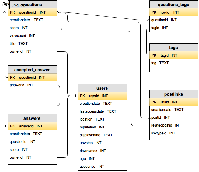
You can download a copy of the SQLite version of the Stack Overflow 2016 database.
Accessing databases in R
The DBI package provides a front-end for manipulating databases from a variety of DBMS (SQLite, MySQL, PostgreSQL, among others). Basically, you tell the package what DBMS is being used on the back-end, link to the actual database, and then you can use the standard functions in the package regardless of the back-end. This is a similar style to how one uses foreach for parallelization.
With SQLite, R processes make calls against the stand-alone SQLite database (.db) file, so there are no SQLite-specific processes. With a client-server DBMS like PostgreSQL, R processes call out to separate Postgres processes; these are started from the overall Postgres background process
You can access and navigate an SQLite database from R as follows.
library(RSQLite)
drv <- dbDriver("SQLite")
dir <- '../data' # relative or absolute path to where the .db file is
dbFilename <- 'stackoverflow-2016.db'
db <- dbConnect(drv, dbname = file.path(dir, dbFilename))
# simple query to get 5 rows from a table
dbGetQuery(db, "select * from questions limit 5")
questionid creationdate score viewcount
1 34552550 2016-01-01 00:00:03 0 108
2 34552551 2016-01-01 00:00:07 1 151
3 34552552 2016-01-01 00:00:39 2 1942
4 34552554 2016-01-01 00:00:50 0 153
5 34552555 2016-01-01 00:00:51 -1 54
title
1 Scope between methods
2 Rails - Unknown Attribute - Unable to add a new field to a form on create/update
3 Selenium Firefox webdriver won't load a blank page after changing Firefox preferences
4 Android Studio styles.xml Error
5 Java: reference to non-finial local variables inside a thread
ownerid
1 5684416
2 2457617
3 5732525
4 5735112
5 4646288## http://www.stat.berkeley.edu/share/paciorek/stackoverflow-2016.dbWe can easily see the tables and their fields:
dbListTables(db)[1] "answers" "cssUsers" "htmlUsers" "questions"
[5] "questions_tags" "tmp" "users" dbListFields(db, "questions")[1] "questionid" "creationdate" "score" "viewcount" "title"
[6] "ownerid" dbListFields(db, "answers")[1] "answerid" "questionid" "creationdate" "score" "ownerid" Here’s how to make a basic SQL query. One can either make the query and get the results in one go or make the query and separately fetch the results. Here we’ve selected the first five rows (and all columns, based on the * wildcard) and brought them into R as a data frame.
results <- dbGetQuery(db, 'select * from questions limit 5')
class(results)
[1] "data.frame"query <- dbSendQuery(db, "select * from questions")
results2 <- fetch(query, 5)
identical(results, results2)[1] TRUEdbClearResult(query) # clear to prepare for another queryTo disconnect from the database:
dbDisconnect(db)Basic SQL for choosing rows and columns from a table
SQL is a declarative language that tells the database system what results you want. The system then parses the SQL syntax and determines how to implement the query.
Note: An imperative language is one where you provide the sequence of commands you want to be run, in order. A declarative language is one where you declare what result you want and rely on the system that interprets the commands how to actually do it. Most of the languages we’re generally familiar with are imperative.
Here are some examples using the Stack Overflow database.
## find the largest viewcounts in the questions table
dbGetQuery(db,
'select title, viewcount from questions order by viewcount desc limit 10')
title
1 How to solve "server DNS address could not be found" error in windows 10?
2 Code signing is required for product type 'Application' in SDK 'iOS 10.0' - StickerPackExtension requires a development team error
3 "Gradle Version 2.10 is required." Error
4 Android- Error:Execution failed for task ':app:transformClassesWithDexForRelease'
5 Fatal error: Uncaught Error: Call to undefined function mysql_connect()
6 Unsupported major.minor version 52.0 in my app
7 Response to preflight request doesn't pass access control check AngularJs
8 NPM vs. Bower vs. Browserify vs. Gulp vs. Grunt vs. Webpack
9 Git refusing to merge unrelated histories
10 "SyntaxError: Unexpected token < in JSON at position 0" in React App
viewcount
1 196469
2 174790
3 134399
4 129874
5 129624
6 127764
7 126752
8 112000
9 109422
10 106995## now get the questions that are viewed the most
dbGetQuery(db, 'select * from questions where viewcount > 100000') questionid creationdate score viewcount
1 35429801 2016-02-16 10:21:09 400 100125
2 37280274 2016-05-17 15:21:49 23 106995
3 37937984 2016-06-21 07:23:00 202 109422
4 35062852 2016-01-28 13:28:39 730 112000
5 35588699 2016-02-23 21:37:06 57 126752
6 35990995 2016-03-14 15:01:17 104 127764
7 34579099 2016-01-03 16:55:16 8 129624
8 35890257 2016-03-09 11:25:05 51 129874
9 34814368 2016-01-15 15:24:36 206 134399
10 37806538 2016-06-14 08:16:21 223 174790
11 36668374 2016-04-16 18:57:19 20 196469
title
1 This action could not be completed. Try Again (-22421)
2 "SyntaxError: Unexpected token < in JSON at position 0" in React App
3 Git refusing to merge unrelated histories
4 NPM vs. Bower vs. Browserify vs. Gulp vs. Grunt vs. Webpack
5 Response to preflight request doesn't pass access control check AngularJs
6 Unsupported major.minor version 52.0 in my app
7 Fatal error: Uncaught Error: Call to undefined function mysql_connect()
8 Android- Error:Execution failed for task ':app:transformClassesWithDexForRelease'
9 "Gradle Version 2.10 is required." Error
10 Code signing is required for product type 'Application' in SDK 'iOS 10.0' - StickerPackExtension requires a development team error
11 How to solve "server DNS address could not be found" error in windows 10?
ownerid
1 5881764
2 4043633
3 2670370
4 2761509
5 2896963
6 1629278
7 3656666
8 1118886
9 3319176
10 1554347
11 1707976Let’s lay out the various verbs in SQL. Here’s the form of a standard query (though the ORDER BY is often omitted and sorting is computationally expensive):
SELECT <column(s)> FROM <table> WHERE <condition(s) on column(s)> ORDER BY <column(s)>SQL keywords are often written in ALL CAPITALS, although I won’t necessarily do that here.
And here is a table of some important keywords:
| Keyword | Usage |
|---|---|
| SELECT | select columns |
| FROM | which table to operate on |
| WHERE | filter (choose) rows satisfying certain conditions |
| LIKE, IN, <, >, ==, etc. | used as part of conditions |
| ORDER BY | sort based on columns |
For comparisons in a WHERE clause, some common syntax for setting conditions includes LIKE (for patterns), =, >, <, >=, <=, !=.
Some other keywords are: DISTINCT, ON, JOIN, GROUP BY, AS, USING, UNION, INTERSECT, SIMILAR TO.
Question: how would we find the oldest users in the database?
Grouping / stratifying
A common pattern of operation is to stratify the dataset, i.e., collect it into mutually exclusive and exhaustive subsets. One would then generally do some operation on each subset. In SQL this is done with the GROUP BY keyword.
Here’s a basic example where we count the occurrences of different tags. Note that we use as to define a name for the new column that is created based on the aggregation operation (count in this case).
dbGetQuery(db, "select tag, count(*) as n from questions_tags
                group by tag order by n desc limit 25")
tag n
1 javascript 290966
2 java 219155
3 android 184272
4 php 177969
5 python 171745
6 c# 163637
7 html 126851
8 jquery 123707
9 ios 95722
10 css 86470
11 angularjs 76951
12 c++ 76260
13 mysql 75458
14 swift 61485
15 sql 58346
16 node.js 52827
17 r 48079
18 arrays 46739
19 json 45250
20 ruby-on-rails 39036
21 sql-server 37077
22 c 36080
23 asp.net 35610
24 excel 29924
25 angular2 28832In general GROUP BY statements will involve some aggregation operation on the subsets. Options include: COUNT, MIN, MAX, AVG, SUM.
If you filter after using GROUP BY, you need to use having instead of where.
Challenge: Write a query that will count the number of answers for each question, returning the most answered questions.
Getting unique results (DISTINCT)
A useful SQL keyword is DISTINCT, which allows you to eliminate duplicate rows from any table (or remove duplicate values when one only has a single column or set of values).
tagNames <- dbGetQuery(db, "select distinct tag from questions_tags")
head(tagNames)
tag
1 c#
2 razor
3 flags
4 javascript
5 rxjs
6 node.jsdbGetQuery(db, "select count(distinct tag) from questions_tags") count(distinct tag)
1 41006Simple SQL joins
Often to get the information we need, we’ll need data from multiple tables. To do this we’ll need to do a database join, telling the database what columns should be used to match the rows in the different tables.
The syntax generally looks like this (again the WHERE and ORDER BY are optional):
SELECT <column(s)> FROM <table1> JOIN <table2> ON <columns to match on> WHERE <condition(s) on column(s)> ORDER BY <column(s)>Let’s see some joins using the different syntax on the Stack Overflow database. In particular let’s select only the questions with the tag python.
result1 <- dbGetQuery(db, "select * from questions join questions_tags
        on questions.questionid = questions_tags.questionid
        where tag = 'python'")
It turns out you can do it without using the JOIN keyword.
result2 <- dbGetQuery(db, "select * from questions, questions_tags
        where questions.questionid = questions_tags.questionid and
        tag = 'python'")

head(result1)
questionid creationdate score viewcount
1 34553559 2016-01-01 04:34:34 3 96
2 34556493 2016-01-01 13:22:06 2 30
3 34557898 2016-01-01 16:36:04 3 143
4 34560088 2016-01-01 21:10:32 1 126
5 34560213 2016-01-01 21:25:26 1 127
6 34560740 2016-01-01 22:37:36 0 455
title
1 Python nested loops only working on the first pass
2 bool operator in for Timestamp in Series does not work
3 Pairwise haversine distance calculation
4 Stopwatch (chronometre) doesn't work
5 How to set the type of a pyqtSignal (variable of class X) that takes a X instance as argument
6 Flask: Peewee model_to_dict helper not working
ownerid questionid tag
1 845642 34553559 python
2 4458602 34556493 python
3 2927983 34557898 python
4 5736692 34560088 python
5 5636400 34560213 python
6 3262998 34560740 pythonidentical(result1, result2)[1] TRUEHere’s a three-way join (using both types of syntax) with some additional use of aliases to abbreviate table names. What does this query ask for?
result1 <- dbGetQuery(db, "select * from
        questions Q
        join questions_tags T on Q.questionid = T.questionid
        join users U on Q.ownerid = U.userid
        where tag = 'python' and
        age > 60")

result2 <- dbGetQuery(db, "select * from
        questions Q, questions_tags T, users U where
        Q.questionid = T.questionid and
        Q.ownerid = U.userid and
        tag = 'python' and
        age > 60")

identical(result1, result2)
[1] TRUEChallenge: Write a query that would return all the answers to questions with the Python tag.
Challenge: Write a query that would return the users who have answered a question with the Python tag.
Temporary tables and views
You can think of a view as a temporary table that is the result of a query and can be used in subsequent queries. In any given query you can use both views and tables. The advantage is that they provide modularity in our querying. For example, if a given operation (portion of a query) is needed repeatedly, one could abstract that as a view and then make use of that view.
Suppose we always want the age and displayname of owners of questions to be readily available. Once we have the view we can query it like a regular table.
dbExecute(db, "create view questionsAugment as select
                questionid, questions.creationdate, score, viewcount,
                title, ownerid, age, displayname
                from questions join users
                on questions.ownerid = users.userid")
[1] 0## you'll see the return value is '0'
dbGetQuery(db, "select * from questionsAugment where age > 70 limit 5") questionid creationdate score viewcount
1 36143022 2016-03-21 22:44:16 2 158
2 40596400 2016-11-14 19:30:32 1 28
3 40612851 2016-11-15 14:51:51 1 32
4 38532865 2016-07-22 18:10:34 0 134
5 36189874 2016-03-23 22:25:56 0 32
title
1 Record aggregate with dynamic choice
2 Why does Xcode report "Variable 'tuple.0' used before being initialized" after I've assigned all elements of a Swift tuple?
3 Converting a Swift array of Ints into an array of its running subtotals
4 Algorithm to generate all permutations of pairs without repetition
5 Mediawiki 1.26.2 upgrade - categories listed in a single column
ownerid age displayname
1 40851 71 Simon Wright
2 74966 71 hkatz
3 74966 71 hkatz
4 98062 71 Rocky Luck
5 332786 71 SakshaleOne use of a view would be to create a mega table that stores all the information from multiple tables in the (unnormalized) form you might have if you simply had one data frame in R or Python.
More on joins
We’ve seen a bunch of joins but haven’t discussed the full taxonomy of types of joins. There are various possibilities for how to do a join depending on whether there are rows in one table that do not match any rows in another table.
Inner joins: In database terminology an inner join is when the result has a row for each match of a row in one table with the rows in the second table, where the matching is done on the columns you indicate. If a row in one table corresponds to more than one row in another table, you get all of the matching rows in the second table, with the information from the first table duplicated for each of the resulting rows. For example in the Stack Overflow data, an inner join of questions and answers would pair each question with each of the answers to that question. However, questions without any answers or (if this were possible) answers without a corresponding question would not be part of the result.
Outer joins: Outer joins add additional rows from one table that do not match any rows from the other table as follows. A left outer join gives all the rows from the first table but only those from the second table that match a row in the first table. A right outer join is the converse, while a full outer join includes at least one copy of all rows from both tables. So a left outer join of the Stack Overflow questions and answers tables would, in addition to the matched questions and their answers, include a row for each question without any answers, as would a full outer join. In this case there should be no answers that do not correspond to question, so a right outer join should be the same as an inner join.
Cross joins: A cross join gives the Cartesian product of the two tables, namely the pairwise combination of every row from each table, analogous to expand.grid() in R. I.e., take a row from the first table and pair it with each row from the second table, then repeat that for all rows from the first table. Since cross joins pair each row in one table with all the rows in another table, the resulting table can be quite large (the product of the number of rows in the two tables). In the Stack Overflow database, a cross join would pair each question with every answer in the database, regardless of whether the answer is an answer to that question.
Simply listing two or more tables separated by commas as we saw earlier is the same as a cross join. Alternatively, listing two or more tables separated by commas, followed by conditions that equate rows in one table to rows in another is equivalent to an inner join.
In general, inner joins can be seen as a form of cross join followed by a condition that enforces matching between the rows of the table. More broadly, here are four equivalent joins that all perform the equivalent of an inner join:
## explicit inner join:
select * from table1 join table2 on table1.id = table2.id
## non-explicit join without JOIN
select * from table1, table2 where table1.id = table2.id
## cross-join followed by matching
select * from table1 cross join table2 where table1.id = table2.id
## explicit inner join with 'using'
select * from table1 join table2 using(id)Challenge: Create a view with one row for every question-tag pair, including questions without any tags.
Challenge: Write a query that would return the displaynames of all of the users who have never posted a question. The NULL keyword will come in handy it’s like ‘NA’ in R. Hint: NULLs should be produced if you do an outer join.
Indexes
An index is an ordering of rows based on one or more fields. DBMS use indexes to look up values quickly, either when filtering (if the index is involved in the WHERE condition) or when doing joins (if the index is involved in the JOIN condition). So in general you want your tables to have indexes.
DBMS use indexing to provide sub-linear time lookup. Without indexes, a database needs to scan through every row sequentially, which is called linear time lookup if there are n rows, the lookup is O(n) in computational cost. With indexes, lookup may be logarithmic O(log(n)) (if using tree-based indexes) or constant time O(1) (if using hash-based indexes). A binary tree-based search is logarithmic; at each step through the tree you can eliminate half of the possibilities.
Here’s how we create an index, with some time comparison for a simple query.
system.time(dbGetQuery(db,
  "select * from questions where viewcount > 10000"))   # 10 seconds
system.time(dbExecute(db,
  "create index count_index on questions (viewcount)")) # 19 seconds
system.time(dbGetQuery(db,
  "select * from questions where viewcount > 10000"))   # 3 seconds
In other contexts, an index can save huge amounts of time. So if you’re working with a database and speed is important, check to see if there are indexes. That said, as seen above it takes time to create the index, so you’d only want to create it if you were doing multiple queries that could take advantage of the index. See the databases tutorial for more discussion of how using indexes in a lookup is not always advantageous.
Creating database tables
One can create tables from within the ‘sqlite’ command line interfaces (discussed in the tutorial), but often one would do this from R or Python. Here’s the syntax from R.
## Option 1: pass directly from CSV to database
dbWriteTable(conn = db, name = "student", value = "student.csv",
             row.names = FALSE, header = TRUE)

## Option 2: pass from data in an R data frame
## create data frame 'student' in some fashion
#student <- data.frame(...)
#student <- read.csv(...)
dbWriteTable(conn = db, name = "student", value = student,
             row.names = FALSE, append = FALSE)
4. Sparsity
A lot of statistical methods are based on sparse matrices. These include:
- Matrices representing the neighborhood structure (i.e., conditional dependence structure) of networks/graphs.
- Matrices representing autoregressive models (neighborhood structure for temporal and spatial data)
- A statistical method called the lasso is used in high-dimensional contexts to give sparse results (sparse parameter vector estimates, sparse covariance matrix estimates)
- There are many others (I’ve been lazy here in not coming up with a comprehensive list, but trust me!)
When storing and manipulating sparse matrices, there is no need to store the zeros, nor to do any computation with elements that are zero.
R, Python, and MATLAB all have functionality for storing and computing with sparse matrices. We’ll see this a bit more in the linear algebra unit.
require(spam)
mat = matrix(rnorm(1e8), 1e4)
mat[mat > (-2)] <- 0
sMat <- as.spam(mat)
print(object.size(mat), units = 'Mb') # 762.9 Mb
print(object.size(sMat), units = 'Mb') # 26 Mb

vec <- rnorm(1e4)
system.time(mat %*% vec)  # 0.385 seconds
system.time(sMat %*% vec) # 0.015 seconds
Here’s a blog post describing the use of sparse matrix manipulations for analysis of the Netflix Prize data.
5. Using statistical concepts to deal with computational bottlenecks
As statisticians, we have a variety of statistical/probabilistic tools that can aid in dealing with big data.
- Usually we take samples because we cannot collect data on the entire population. But we can just as well take a sample because we don’t have the ability to process the data from the entire population. We can use standard uncertainty estimates to tell us how close to the true quantity we are likely to be. And we can always take a bigger sample if we’re not happy with the amount of uncertainty.
- There are a variety of ideas out there for making use of sampling to address big data challenges. One idea (due in part to Prof. Michael Jordan here in Statistics/EECS) is to compute estimates on many (relatively small) bootstrap samples from the data (cleverly creating a reduced-form version of the entire dataset from each bootstrap sample) and then combine the estimates across the samples. Here’s the arXiv paper on this topic, also published as Kleiner et al. in Journal of the Royal Statistical Society (2014) 76:795.
- Randomized algorithms: there has been a lot of attention recently to algorithms that make use of randomization. E.g., in optimizing a likelihood, you might choose the next step in the optimization based on random subset of the data rather than the full data. Or in a regression context you might choose a subset of rows of the design matrix (the matrix of covariates) and corresponding observations, weighted based on the statistical leverage ([recall the discussion of regression diagnostics in a regression course) of the observations. Here’s another arXiv paper that provides some ideas in this area.