# To answer this problem, I wrote the code below which does x, y, and z...
# and this comment should instead be in the text above the code chunk :(
how_to_lose_points <- function(...) { ... }PS3 code review
Overview
In section this week we will do a paired code review for Problem 1 of PS3.
In order for this to be beneficial, you will need to be as honest with your partner as possible (while staying respectful). If something is actually hard to follow, tell them! If you thought that something they did was clever, also tell them!
Instructions
We will break up into pairs of 2 (with a possible group of 3 if necessary). Please open up the PDF you submitted.
Next, you will spend ~15 minutes reading one partner’s code, asking questions to the person whose code you are reviewing. You will then switch roles so that the reviewer becomes the reviewee.
Finally, each of you will fill out the survey at the following link: tinyurl.com/stat243-2022-lab5, where you will summarize the differences between your work and and your partner’s work, noting anything that was particularly novel to you. You will need to log in with your Berkeley account to access this survey.
The survey response is worth 1 point, similar to in class group work or the unit check ins, and will be graded. You will receive credit as long as your response is thoughtful (e.g. at least a couple of sentences). If you choose not to come to section, please find a partner or two on your own to do the paired review with and submit the survey by Wednesday Oct. 5 at 5:59pm to receive credit.
Some Guiding Questions
Is the code visually easy to break apart? Can you see the entire body of the functions without scrolling up/down left/right? The general rule-of-thumb is no more than 80 in either direction (80 character width, 80 lines; the first restriction should be practiced more religiously).
Are the data structures easy to parse? Do you understand what information is in which objects? Is the type of data appropriate?
Are the functions easy to parse? Is it clear what they are doing, what information is being passed to each function, and what the return value/objects are?
Look at the regex. Are there any edge cases that were missed? Was anything handled particularly well? Any novel expressions that you didn’t think of?
Look at the plots. Are they well labeled? Is it easy to read information from them? Do they provide an assurance that the code is running correctly? Was there anything particularly neat about your partner’s solution?
EXTRA. Look at Problem 2, compare/contrast your approaches to OOP. Explain the logic behind your design.
General notes about homeworks
Below are some notes to keep in mind when doing your problem sets.
Address All Aspects of the Problems
You have to answer the questions on the homework, unless the instructions say otherwise. When in doubt, please post to Ed Discussion!
Do whatever you’d like beyond that and be as creative as you wish, but you must answer the questions that were asked. This includes all parts of a written response question. If you do not answer these, you are throwing away points.
Code Should be Preceded By Introductory Text
For each sub-problem where code is required, please include an introduction to in the text before presenting any code. This should include a brief summary of what the code does and how you approached the solution, plus any relevant challenges you faced. This doesn’t have to be very long, but it should have some substance.
If there’s a natural stopping point in your code – e.g., between separate functions, after you’ve accomplished some task(s), or somewhere you want to highlight what you just did – then feel free to break longer code chunks up with some text if you think it will help with readability / flow of your document. However, good code quality and substantive code comments will often suffice.
Code comments are not a replacement for the introductory text
a. How to lose Presentation points
Include Your Code
Most people include it as they go along, which is fine. If you find that messy, put an appendix at the end with all of the function definitions. This applies to code for plots as well.
Include Relevant Outputs
Where appropriate, include some sample outputs from your code. You don’t have to do this for every single function, but be sure to give outputs if the question asks for it to avoid points off, e.g. “print out or plot the number of chunks for the candidates” or “report the number of observations in each year by printing the information to the screen”.
If outputs are long and you can’t truncate them, then create an appendix section at the end of your document and put them there, with a subheading for the relevant problem. Please also be sure to include a note that you did so in the text, e.g. “The output can be found in the Appendix.”
Avoid Unnecessary Outputs
Please use suppressPackageStartupMessages() or set warning = FALSE and message = FALSE in a code chunk that only loads the packages. Please on’t use these chunk options on other chunks. If something is going wrong ou need to fix it, as opposed to not printing the warning.
Use Good Formatting to Make Clear What Problem You’re Answering
You have the power of Markdown in your hands, so use it! While you’re free to use the .Rmd source code for the problem set instructions as a template, the instructions are written as a list, and .Rmd is finicky when adding text or code chunks between sequential list items.
It can often be less error-prone to start a new .Rmd from scratch and just use header tags like # (top level section) and ## (second level section) to separate your problems and sub-problems.
For example:
# Problem 1: Assertions and testing

## a. Assertions

In the function below, I added an assertion to check for...
which guards against... and gives helpful feedback to the user
telling them to...
Note that you have to include a space between the final # and the header text, or the header won’t render correctly, e.g.:
#Headerproduces the following non-header text:
#Header
If you’re having trouble with Markdown, see 2.5 Markdown syntax from the R Markdown: The Definitive Guide book.
A Couple of Useful Tools in RStudio
You can autoindent your code in RStudio using Command or Ctrl + I. You can also autoformat your code with Shift + Command or Ctrl + A. There are some other useful shortcuts in the Code menu.
Extra Credit
This is something additional, above and beyond the basic homework. Repeating the analysis already performed, but with different parameters, is not novel.
Code Testing
You should have already tested all aspects of your R code before you submit it. Your code should run properly if you restart RStudio and render your .Rmd. I have seen several assignments where students renamed a variable at the last second which causes their code to break, are referencing a global variable that doesn’t exist in the .Rmd, etc. which tells me they did not fully test that their code works before submitting. When reasonable, the functions you create should have a set of small but thoughtful examples showing that the code works as expected.
Simple is Often Better
You should always be thinking of ways to make your code as simple as possible (while maintaining correctness, numerical precision, speed, etc.). For example, the following three chunks of code all do the same thing:
total <- 0
for (i in 1:length(x)) {
    total <- total + x[i]
}
total / length(x)sum(x) / length(x)mean(x)But the third option is preferred. Simple code helps with debugging (as there are fewer lines of code to check), improves readability (both for yourself and others), and can often (though not always) result in faster code.
Plots and Comments
Plots need to have a title, axis labels, and a key if there are several types of data. Both code and comment lines should be ~80 characters in length, e.g.:
####################
# Wrap your comments
####################

# This is a bad comment
# Lorem ipsum dolor sit amet, consectetur adipiscing elit, sed do eiusmod tempor incididunt ut labore et dolore magna aliqua. Ut enim ad minim veniam, quis nostrud exercitation ullamco laboris nisi ut aliquip ex ea commodo consequat. Duis aute irure dolor in reprehenderit in voluptate velit esse cillum dolore eu fugiat nulla pariatur. Excepteur sint occaecat cupidatat non proident, sunt in culpa qui officia deserunt mollit anim id est laborum.

# This is a good comment
# Lorem ipsum dolor sit amet, consectetur adipiscing elit, sed do eiusmod
# tempor incididunt ut labore et dolore magna aliqua. Ut enim ad minim
# veniam, quis nostrud exercitation ullamco laboris nisi ut aliquip ...etc

###############
# Good plotting
###############

# set things up
n <- 50
x <- 1:n
y <- runif(n = n, min = 0, max = 10)

col_factor <- sample(x = c(1, 2), size = n, replace = T, prob = c(1, 2))

df <- data.frame(x, y, color = as.factor(col_factor))

# make the plot
ggplot(df, aes(x = x, y = y)) +
  geom_point(aes(color = color), size = 3) +
  geom_line() +
  theme_bw() +
  labs(x = "Label related to data", y = "Label related to data") +
  ggtitle("Short but informative title") +
  scale_color_discrete(name = "Group designation") +
  theme(legend.position = c(1, 1),
        legend.justification = c(1, 1),
        legend.background = element_blank(),
        legend.box.background = element_rect(colour = "black")) +
  ylim(0, 13)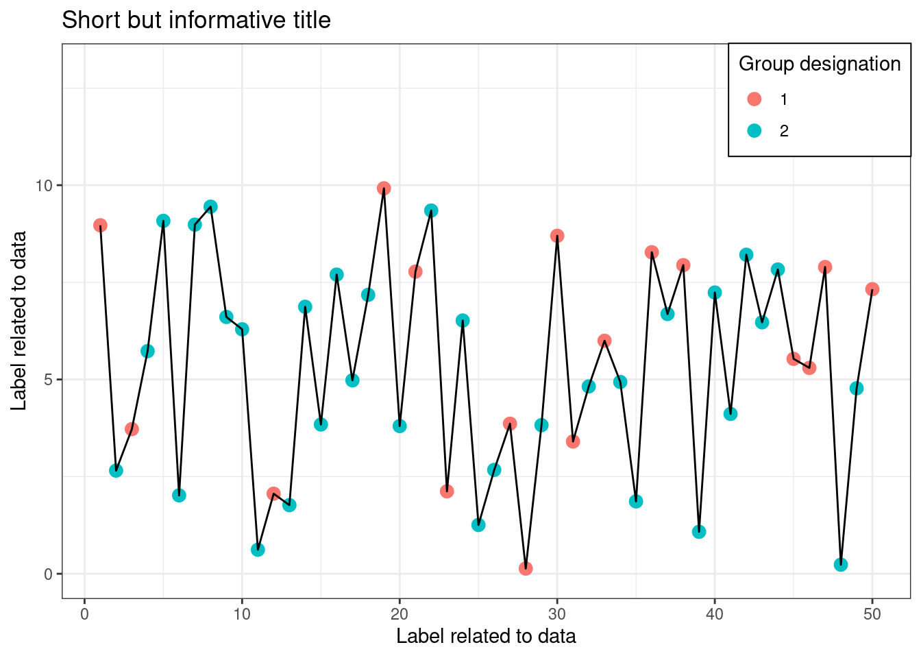
Vectorization
“Vectorization” in R implies using functions that naturally operate over vector inputs, rather than processing each element one at a time. This ends up being faster because, under the hood, vectorized functions in R actually call corresponding code written in C, and the C code itself uses a loop that runs much more quickly than an equivalent loop in R would. But to do that, it needs to receive the full vector all at once.
R is vectorized in many basic mathematical operations (addition, subtraction, multiplication, division, etc.) and any other functions have built-in vectorization as well. Some functions – like those for linear algebra – even use highly optimized parallel routines in C, adding further speedups. So when operating on large vectors or matrices, be sure to check the documentation to see if there is a vectorized function that you can use to your advantage.
#####################
# vectorized division
#####################

x <- 1:100
y <- 100:1

a_div <- mapply(FUN = "/", x, y)
v_div <- x / y

all.equal(a_div, v_div)
[1] TRUEidentical(a_div, v_div)[1] TRUE########################
# vectorized multinomial
########################
probs <- matrix(data = c(0.1,0.1,0.8, 1/3,1/3,1/3), nrow = 2, byrow = T)
set.seed(0)
a_mnom <- t(apply(X = probs, MARGIN = 1, FUN = rmultinom,
n = 1, size = 100))
set.seed(0)
v_mnom <- extraDistr::rmnom(n = 2, size = 100, prob = probs)
all.equal(a_mnom, v_mnom)[1] TRUEidentical(a_mnom, v_mnom) # why false?[1] FALSE# short benchmark
microbenchmark::microbenchmark(
"apply" = apply(X = probs, MARGIN = 1,
FUN = rmultinom, n = 1, size = 100),
"vector" = extraDistr::rmnom(n = 2, size = 100,
prob = probs),
times = 100)Unit: microseconds
expr min lq mean median uq max neval cld
apply 36.720 37.6400 39.77439 38.728 39.49 102.926 100 b
vector 5.639 6.1305 7.42927 7.014 8.30 23.061 100 a If you want to learn a bit more about vectorization, check out 24.5 Vectorize in the AdvancedR book.