import dask
dask.config.set(scheduler='threads', num_workers = 4)
import dask.dataframe as ddf
path = '/scratch/users/paciorek/243/AirlineData/csvs/'
air = ddf.read_csv(path + '*.csv.bz2',
      compression = 'bz2',
      encoding = 'latin1', # (unexpected) latin1 value(s) in TailNum field in 2001
      dtype = {'Distance': 'float64', 'CRSElapsedTime': 'float64',
      'TailNum': 'object', 'CancellationCode': 'object', 'DepDelay': 'float64'})
# specify some dtypes so Pandas doesn't complain about column type heterogeneity
airBig data and databases
References:
- Tutorial on parallel processing using Python’s Dask and R’s future packages
- Tutorial on working with large datasets in SQL, R, and Python
- Murrell: Introduction to Data Technologies
- Adler: R in a Nutshell
- Spark Programming Guide
I’ve also pulled material from a variety of other sources, some mentioned in context below.
Note that for a lot of the demo code I ran the code separately from rendering this document because of the time involved in working with large datasets.
We’ll focus on Dask and databases/SQL in this Unit. The material on using Spark is provided for reference, but you’re not responsible for that material. If you’re interested in working with big datasets in R or with tools other than Dask in Python, there is some material in the tutorial on working with large datasets.
1. A few preparatory notes
An editorial on ‘big data’
‘Big data’ was trendy these days, though I guess it’s not quite the buzzword/buzzphrase that it was a few years ago, given the AI/ML revolution, but of course that revolution is largely based on having massive datasets available online.
Personally, I think some of the hype around giant datasets is justified and some is hype. Large datasets allow us to address questions that we can’t with smaller datasets, and they allow us to consider more sophisticated (e.g., nonlinear) relationships than we might with a small dataset. But they do not directly help with the problem of correlation not being causation. Having medical data on every American still doesn’t tell me if higher salt intake causes hypertension. Internet transaction data does not tell me if one website feature causes increased viewership or sales. One either needs to carry out a designed experiment or think carefully about how to infer causation from observational data. Nor does big data help with the problem that an ad hoc ‘sample’ is not a statistical sample and does not provide the ability to directly infer properties of a population. Consider the immense difficulties we’ve seen in answering questions about Covid despite large amounts of data, because it is incomplete/non-representative. A well-chosen smaller dataset may be much more informative than a much larger, more ad hoc dataset. However, having big datasets might allow you to select from the dataset in a way that helps get at causation or in a way that allows you to construct a population-representative sample. Finally, having a big dataset also allows you to do a large number of statistical analyses and tests, so multiple testing is a big issue. With enough analyses, something will look interesting just by chance in the noise of the data, even if there is no underlying reality to it.
Different people define the ‘big’ in big data differently. One definition involves the actual size of the data, and in some cases the speed with which it is collected. Our efforts here will focus on dataset sizes that are large for traditional statistical work but would probably not be thought of as large in some contexts such as Google or the US National Security Agency (NSA). Another definition of ‘big data’ has more to do with how pervasive data and empirical analyses backed by data are in society and not necessarily how large the actual dataset size is.
Logistics and data size
One of the main drawbacks with Python (and R) in working with big data is that all objects are stored in memory, so you can’t directly work with datasets that are more than 1-20 Gb or so, depending on the memory on your machine.
The techniques and tools discussed in this Unit (apart from the section on MapReduce/Spark) are designed for datasets in the range of gigabytes to tens of gigabytes, though they may scale to larger if you have a machine with a lot of memory or simply have enough disk space and are willing to wait. If you have 10s of gigabytes of data, you’ll be better off if your machine has 10s of GBs of memory, as discussed in this Unit.
If you’re scaling to 100s of GBs, terabytes or petabytes, tools such as carefully-administered databases, cloud-based tools such as provided by AWS and Google Cloud Platform, and Spark or other such tools are probably your best bet.
Note: in handling big data files, it’s best to have the data on the local disk of the machine you are using to reduce traffic and delays from moving data over the network.
What we already know about handling big data!
UNIX operations are generally very fast, so if you can manipulate your data via UNIX commands and piping, that will allow you to do a lot. We’ve already seen UNIX commands for extracting columns. And various commands such as grep, head, tail, etc. allow you to pick out rows based on certain criteria. As some of you have done in problem sets, one can use awk to extract rows. So basic shell scripting may allow you to reduce your data to a more manageable size.
The tool GNU parallel allows you to parallelize operations from the command line and is commonly used in working on Linux clusters.
And don’t forget simple things. If you have a dataset with 30 columns that takes up 10 Gb but you only need 5 of the columns, get rid of the rest and work with the smaller dataset. Or you might be able to get the same information from a random sample of your large dataset as you would from doing the analysis on the full dataset. Strategies like this will often allow you to stick with the tools you already know.
Also, remember that we can often store data more compactly in binary formats than in flat text (e.g., csv) files.
Finally, for many applications, storing large datasets in a standard database will work well.
2. MapReduce, Dask, Hadoop, and Spark
Traditionally, high-performance computing (HPC) has concentrated on techniques and tools for message passing such as MPI and on developing efficient algorithms to use these techniques. In the last 20 years, focus has shifted to technologies for processing large datasets that are distributed across multiple machines but can be manipulated as if they are one dataset.
Two commonly-used tools for doing this are Spark and Python’s Dask package. We’ll cover Dask.
Overview
A basic paradigm for working with big datasets is the MapReduce paradigm. The basic idea is to store the data in a distributed fashion across multiple nodes and try to do the computation in pieces on the data on each node. Results can also be stored in a distributed fashion.
A key benefit of this is that if you can’t fit your dataset on disk on one machine you can on a cluster of machines. And your processing of the dataset can happen in parallel. This is the basic idea of MapReduce.
The basic steps of MapReduce are as follows:
- read individual data objects (e.g., records/lines from CSVs or individual data files)
- map: create key-value pairs using the inputs (more formally, the map step takes a key-value pair and returns a new key-value pair)
- reduce: for each key, do an operation on the associated values and create a result - i.e., aggregate within the values assigned to each key
- write out the {key,result} pair
A similar paradigm that is implemented in pandas and dplyr is the split-apply-combine strategy.
A few additional comments. In our map function, we could exclude values or transform them in some way, including producing multiple records from a single record. And in our reduce function, we can do more complicated analysis. So one can actually do fairly sophisticated things within what may seem like a restrictive paradigm. But we are constrained such that in the map step, each record needs to be treated independently and in the reduce step each key needs to be treated independently. This allows for the parallelization.
One important note is that any operations that require moving a lot of data between the workers can take a long time. (This is sometimes called a shuffle.) This could happen if, for example, you computed the median value within each of many groups if the data for each group are spread across the workers. In contrast, if we compute the mean or sum, one can compute the partial sums on each worker and then just add up the partial sums.
Note that as discussed in Unit 5 the concepts of map and reduce are core concepts in functional programming, and of course Python provides the map function.
Hadoop is an infrastructure for enabling MapReduce across a network of machines. The basic idea is to hide the complexity of distributing the calculations and collecting results. Hadoop includes a file system for distributed storage (HDFS), where each piece of information is stored redundantly (on multiple machines). Calculations can then be done in a parallel fashion, often on data in place on each machine thereby limiting the amount of communication that has to be done over the network. Hadoop also monitors completion of tasks and if a node fails, it will redo the relevant tasks on another node. Hadoop is based on Java. Given the popularity of Spark, I’m not sure how much usage these approaches currently see. Setting up a Hadoop cluster can be tricky. Hopefully if you’re in a position to need to use Hadoop, it will be set up for you and you will be interacting with it as a user/data analyst.
Ok, so what is Spark? You can think of Spark as in-memory Hadoop. Spark allows one to treat the memory across multiple nodes as a big pool of memory. Therefore, Spark should be faster than Hadoop when the data will fit in the collective memory of multiple nodes. In cases where it does not, Spark will make use of the HDFS (and generally, Spark will be reading the data initially from HDFS.) While Spark is more user-friendly than Hadoop, there are also some things that can make it hard to use. Setting up a Spark cluster also involves a bit of work, Spark can be hard to configure for optimal performance, and Spark calculations have a tendency to fail (often involving memory issues) in ways that are hard for users to debug.
Using Dask for big data processing
Unit 6 on parallelization gives an overview of using Dask for flexible parallelization on different kinds of computational resources (in particular, parallelizing across multiple cores on one machine versus parallelizing across multiple cores across multiple machines/nodes).
Here we’ll see the use of Dask to work with distributed datasets. Dask can process datasets (potentially very large ones) by parallelizing operations across subsets of the data using multiple cores on one or more machines.
Like Spark, Dask automatically reads data from files in parallel and operates on chunks (also called partitions or shards) of the full dataset in parallel. There are two big advantages of this:
- You can do calculations (including reading from disk) in parallel because each worker will work on a piece of the data.
- When the data is split across machines, you can use the memory of multiple machines to handle much larger datasets than would be possible in memory on one machine. That said, Dask processes the data in chunks, so one often doesn’t need a lot of memory, even just on one machine.
While reading from disk in parallel is a good goal, if all the data are on one hard drive, there are limitations on the speed of reading the data from disk because of having multiple processes all trying to access the disk at once. Supercomputing systems will generally have parallel file systems that support truly parallel reading (and writing, i.e., parallel I/O). Hadoop/Spark deal with this by distributing across multiple disks, generally one disk per machine/node.
Because computations are done in external compiled code (e.g., via numpy) it’s effective to use the threads scheduler when operating on one node to avoid having to copy and move the data.
Dask dataframes (pandas)
Dask dataframes are Pandas-like dataframes where each dataframe is split into groups of rows, stored as smaller Pandas dataframes.
One can do a lot of the kinds of computations that you would do on a Pandas dataframe on a Dask dataframe, but many operations are not possible. See here.
By default dataframes are handled by the threads scheduler. (Recall we discussed Dask’s various schedulers in Unit 6.)
Here’s an example of reading from a dataset of flight delays (about 11 GB data). You can get the data here.
Dask will reads the data in parallel from the various .csv.bz2 files (unzipping on the fly), but note the caveat in the previous section about the possibilities for truly parallel I/O.
However, recall that Dask uses delayed evaluation. In this case, the reading is delayed until compute() is called. For that matter, the various other calculations (max, groupby, mean) shown below are only done after compute() is called.
import time

t0 = time.time()
air.DepDelay.max().compute()   # this takes a while
print(time.time() - t0)

t0 = time.time()
air.DepDelay.mean().compute()   # this takes a while
print(time.time() - t0)

air.DepDelay.median().compute()
We’ll discuss in class why Dask won’t do the median. Consider the discussion about moving data in the earlier section on MapReduce.
Next let’s see a full split-apply-combine (aka MapReduce) type of analysis.
sub = air[(air.UniqueCarrier == 'UA') & (air.Origin == 'SFO')]
byDest = sub.groupby('Dest').DepDelay.mean()
results = byDest.compute()            # this takes a while too
results
You should see this:
    Dest
    ACV 26.200000
    BFL 1.000000
    BOI 12.855069
    BOS 9.316795
    CLE 4.000000
    ...
Note: calling compute twice is a bad idea as Dask will read in the data twice - more on this in a bit.
Warning Think carefully about the size of the result from calling
compute. The result will be returned as a standard Python object, not distributed across multiple workers (and possibly machines), and with the object entirely in memory. It’s easy to accidentally return an entire giant dataset.
Dask bags
Bags are like lists but there is no particular ordering, so it doesn’t make sense to ask for the i’th element.
You can think of operations on Dask bags as being like parallel map operations on lists in Python or R.
By default bags are handled via the processes scheduler.
Let’s see some basic operations on a large dataset of Wikipedia log files. You can get a subset of the Wikipedia data here.
Here we again read the data in (which Dask will do in parallel):
import dask.multiprocessing
dask.config.set(scheduler='processes', num_workers = 4)
import dask.bag as db
## This is the full data
## path = '/scratch/users/paciorek/wikistats/dated_2017/'
## For demo we'll just use a small subset
path = '/scratch/users/paciorek/wikistats/dated_2017_small/dated/'
wiki = db.read_text(path + 'part-0*gz')
Here we’ll just count the number of records.
import time
t0 = time.time()
wiki.count().compute()
time.time() - t0   # 136 sec. for full data
And here is a more realistic example of filtering (subsetting).
import re
def find(line, regex = 'Armenia'):
    vals = line.split(' ')
    if len(vals) < 6:
        return(False)
    tmp = re.search(regex, vals[3])
    if tmp is None:
        return(False)
    else:
        return(True)


wiki.filter(find).count().compute()
armenia = wiki.filter(find)
smp = armenia.take(100) ## grab a handful as proof of concept
smp[0:5]
Note that it is quite inefficient to do the find() (and implicitly reading the data in) and then compute on top of that intermediate result in two separate calls to compute(). Rather, we should set up the code so that all the operations are set up before a single call to compute(). This is discussed in detail in the Dask/future tutorial.
Since the data are just treated as raw strings, we might want to introduce structure by converting each line to a tuple and then converting to a data frame.
def make_tuple(line):
    return(tuple(line.split(' ')))

dtypes = {'date': 'object', 'time': 'object', 'language': 'object',
'webpage': 'object', 'hits': 'float64', 'size': 'float64'}

## Let's create a Dask dataframe.
## This will take a while if done on full data.
df = armenia.map(make_tuple).to_dataframe(dtypes)
type(df)

## Now let's actually do the computation, returning a Pandas df
result = df.compute()
type(result)
result[0:5]
Dask arrays (numpy)
Dask arrays are numpy-like arrays where each array is split up by both rows and columns into smaller numpy arrays.
One can do a lot of the kinds of computations that you would do on a numpy array on a Dask array, but many operations are not possible. See here.
By default arrays are handled via the threads scheduler.
Non-distributed arrays
Let’s first see operations on a single node, using a single 13 GB two-dimensional array. Again, Dask uses lazy evaluation, so creation of the array doesn’t happen until an operation requiring output is done.
import dask
dask.config.set(scheduler = 'threads', num_workers = 4)
import dask.array as da
x = da.random.normal(0, 1, size=(40000,40000), chunks=(10000, 10000))
# square 10k x 10k chunks
mycalc = da.mean(x, axis = 1)  # by row
import time
t0 = time.time()
rs = mycalc.compute()
time.time() - t0  # 41 sec.
For a row-based operation, we would presumably only want to chunk things up by row, but this doesn’t seem to actually make a difference, presumably because the mean calculation can be done in pieces and only a small number of summary statistics moved between workers.
import dask
dask.config.set(scheduler='threads', num_workers = 4)
import dask.array as da
# x = da.from_array(x, chunks=(2500, 40000))  # adjust chunk size of existing array
x = da.random.normal(0, 1, size=(40000,40000), chunks=(2500, 40000))
mycalc = da.mean(x, axis = 1)  # row means
import time
t0 = time.time()
rs = mycalc.compute()
time.time() - t0   # 42 sec.
Of course, given the lazy evaluation, this timing comparison is not just timing the actual row mean calculations.
But this doesn’t really clarify the story…
import dask
dask.config.set(scheduler='threads', num_workers = 4)
import dask.array as da
import numpy as np
import time
t0 = time.time()
x = np.random.normal(0, 1, size=(40000,40000))
time.time() - t0   # 110 sec.
# for some reason the from_array and da.mean calculations are not done lazily here
t0 = time.time()
dx = da.from_array(x, chunks=(2500, 40000))
time.time() - t0   # 27 sec.
t0 = time.time()
mycalc = da.mean(x, axis = 1)  # what is this doing given .compute() also takes time?
time.time() - t0   # 28 sec.
t0 = time.time()
rs = mycalc.compute()
time.time() - t0   # 21 sec.
Dask will avoid storing all the chunks in memory. (It appears to just generate them on the fly.) Here we have an 80 GB array but we never use more than a few GB of memory (based on top or free -h).
import dask
dask.config.set(scheduler='threads', num_workers = 4)
import dask.array as da
x = da.random.normal(0, 1, size=(100000,100000), chunks=(10000, 10000))
mycalc = da.mean(x, axis = 1)  # row means
import time
t0 = time.time()
rs = mycalc.compute()
time.time() - t0   # 205 sec.
rs[0:5]
Distributed arrays
Using arrays distributed across multiple machines should be straightforward based on using Dask distributed. However, one would want to be careful about creating arrays by distributing the data from a single Python process as that would involve copying between machines.
3. Databases
This material is drawn from the tutorial on Working with large datasets in SQL, R, and Python, though I won’t hold you responsible for all of the database/SQL material in that tutorial, only what appears here in this Unit.
Overview
Basically, standard SQL databases are relational databases that are a collection of rectangular format datasets (tables, also called relations), with each table similar to R or Pandas data frames, in that a table is made up of columns, which are called fields or attributes, each containing a single type (numeric, character, date, currency, enumerated (i.e., categorical), …) and rows or records containing the observations for one entity. Some of the tables in a given database will generally have fields in common so it makes sense to merge (i.e., join) information from multiple tables. E.g., you might have a database with a table of student information, a table of teacher information and a table of school information, and you might join student information with information about the teacher(s) who taught the students. Databases are set up to allow for fast querying and merging (called joins in database terminology).
Memory and disk use
Formally, databases are stored on disk, while Python and R store datasets in memory. This would suggest that databases will be slow to access their data but will be able to store more data than can be loaded into an Python or R session. However, databases can be quite fast due in part to disk caching by the operating system as well as careful implementation of good algorithms for database operations.
Interacting with a database
You can interact with databases in a variety of database systems (DBMS=database management system). Some popular systems are SQLite, DuckDB, MySQL, PostgreSQL, Oracle and Microsoft Access. We’ll concentrate on accessing data in a database rather than management of databases. SQL is the Structured Query Language and is a special-purpose high-level language for managing databases and making queries. Variations on SQL are used in many different DBMS.
Queries are the way that the user gets information (often simply subsets of tables or information merged across tables). The result of an SQL query is in general another table, though in some cases it might have only one row and/or one column.
Many DBMS have a client-server model. Clients connect to the server, with some authentication, and make requests (i.e., queries).
There are often multiple ways to interact with a DBMS, including directly using command line tools provided by the DBMS or via Python or R, among others.
We’ll concentrate on SQLite (because it is simple to use on a single machine). SQLite is quite nice in terms of being self-contained - there is no server-client model, just a single file on your hard drive that stores the database and to which you can connect to using the SQLite shell, R, Python, etc. However, it does not have some useful functionality that other DBMS have. For example, you can’t use ALTER TABLE to modify column types or drop columns.
A good alternative to SQLite that I encourage you to consider is DuckDB. DuckDB stores data column-wise, which can lead to big speedups when doing queries operating on large portions of tables (so-called “online analytical processing” (OLAP)). Another nice feature of DuckDB is that it can interact with data on disk without always having to read all the data into memory. In fact, ideally we’d use it for this class, but I haven’t had time to create a DuckDB version of the StackOverflow database.
Database schema and normalization
To truly leverage the conceptual and computational power of a database you’ll want to have your data in a normalized form, which means spreading your data across multiple tables in such a way that you don’t repeat information unnecessarily.
The schema is the metadata about the tables in the database and the fields (and their types) in those tables.
Let’s consider this using an educational example. Suppose we have a school with multiple teachers teaching multiple classes and multiple students taking multiple classes. If we put this all in one table organized per student, the data might have the following fields:
- student ID
- student grade level
- student name
- class 1
- class 2
- …
- class n
- grade in class 1
- grade in class 2
- …
- grade in class n
- teacher ID 1
- teacher ID 2
- …
- teacher ID n
- teacher name 1
- teacher name 2
- …
- teacher name n
- teacher department 1
- teacher department 2
- …
- teacher department n
- teacher age 1
- teacher age 2
- …
- teacher age n
There are a lot of problems with this:
- A lot of information is repeated across rows (e.g., teacher age for students who have the same teacher) - this is a waste of space - it is hard/error-prone to update values in the database (e.g., after a teacher’s birthday), because a given value needs to be updated in multiple places
- There are potentially a lot of empty cells (e.g., for a student who takes fewer than ‘n’ classes). This will generally result in a waste of space.
- It’s hard to see the information that is not organized uniquely by row – i.e., it’s much easier to understand the information at the student level than the teacher level
- We have to know in advance how big ‘n’ is. Then if a single student takes more than ‘n’ classes, the whole database needs to be restructured.
It would get even worse if there was a field related to teachers for which a given teacher could have multiple values (e.g., teachers could be in multiple departments). This would lead to even more redundancy - each student-class-teacher combination would be crossed with all of the departments for the teacher (so-called multivalued dependency in database theory).
An alternative organization of the data would be to have each row represent the enrollment of a student in a class.
- student ID
- student name
- class
- grade in class
- student grade level
- teacher ID
- teacher department
- teacher age
This has some advantages relative to our original organization in terms of not having empty cells, but it doesn’t solve the other three issues above.
Instead, a natural way to order this database is with the following four tables.
- Student
- ID
- name
- grade_level
- Teacher
- ID
- name
- department
- age
- Class
- ID
- topic
- class_size
- teacher_ID
- ClassAssignment
- student_ID
- class_ID
- grade
The ClassAssignment table has one row per student-class pair. Having a table like this handles “ragged” data where the number of observations per unit (in this case classes per student) varies. Using such tables is a common pattern when considering how to normalize a database. It’s also a core part of the idea of “tidy data” and data in long format, seen in the tidyr package.
Then we do queries to pull information from multiple tables. We do the joins based on keys, which are the fields in each table that allow us to match rows from different tables.
(That said, if all anticipated uses of a database will end up recombining the same set of tables, we may want to have a denormalized schema in which those tables are actually combined in the database. It is possible to be too pure about normalization! We can also create a virtual table, called a view, as discussed later.)
Keys
A key is a field or collection of fields that give(s) a unique value for every row/observation. A table in a database should then have a primary key that is the main unique identifier used by the DBMS. Foreign keys are columns in one table that give the value of the primary key in another table. When information from multiple tables is joined together, the matching of a row from one table to a row in another table is generally done by equating the primary key in one table with a foreign key in a different table.
In our educational example, the primary keys would presumably be: Student.ID, Teacher.ID, Class.ID, and for ClassAssignment a primary key made of two fields: {ClassAssignment.studentID, ClassAssignment.class_ID}.
Some examples of foreign keys would be:
student_IDas the foreign key inClassAssignmentfor joining withStudentonStudent.IDteacher_IDas the foreign key inClassfor joining withTeacherbased onTeacher.IDclass_IDas the foreign key inClassAssignmentfor joining withClassbased onClass.ID
Queries that join data across multiple tables
Suppose we want a result that has the grades of all students in 9th grade. For this we need information from the Student table (to determine grade level) and information from the ClassAssignment table (to determine the class grade). More specifically we need a query that:
- joins
StudentwithClassAssignmentbased on matching rows inStudentwith rows inClassAssignmentwhereStudent.IDis the same asClassAssignment.student_IDand - filters the rows based on
Student.grade_level:
SELECT Student.ID, grade FROM Student, ClassAssignment WHERE
  Student.ID = ClassAssignment.student_ID and Student.grade_level = 9;
Note that the query is a join (specifically an inner join), which is like merge() (or dplyr::join) in R. We don’t specifically use the JOIN keyword, but one could do these queries explicitly using JOIN, as we’ll see later.
Stack Overflow metadata example
I’ve obtained data from Stack Overflow, the popular website for asking coding questions, and placed it into a normalized database. The SQLite version has metadata (i.e., it lacks the actual text of the questions and answers) on all of the questions and answers posted in 2021.
We’ll explore SQL functionality using this example database.
Now let’s consider the Stack Overflow data. Each question may have multiple answers and each question may have multiple (topic) tags.
If we tried to put this into a single table, the fields could look like this if we have one row per question:
- question ID
- ID of user submitting question
- question title
- tag 1
- tag 2
- …
- tag n
- answer 1 ID
- ID of user submitting answer 1
- age of user submitting answer 1
- name of user submitting answer 1
- answer 2 ID
- ID of user submitting answer 2
- age of user submitting answer 2
- name of user submitting answer 2
- …
or like this if we have one row per question-answer pair:
- question ID
- ID of user submitting question
- question title
- tag 1
- tag 2
- …
- tag n
- answer ID
- ID of user submitting answer
- age of user submitting answer
- name of user submitting answer
As we’ve discussed neither of those schema is particularly desirable.
Challenge: How would you devise a schema to normalize the data. I.e., what set of tables do you think we should create?
You can view one reasonable schema. The lines between tables indicate the relationship of foreign keys in one table to primary keys in another table. The schema in the actual database of Stack Overflow data we’ll use in the examples here is similar to but not identical to that.
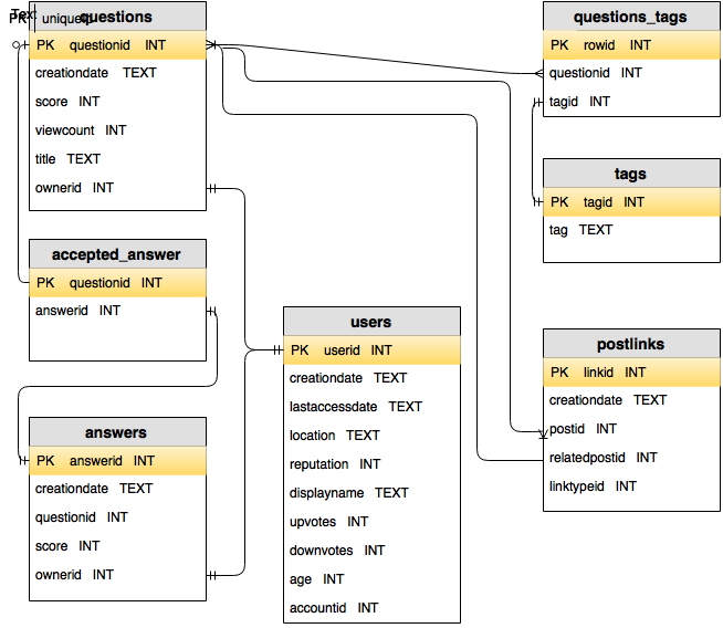
You can download a copy of the SQLite version of the Stack Overflow 2021 database.
Accessing databases in Python
Python provides a variety of front-end packages for manipulating databases from a variety of DBMS (SQLite, DuckDB, MySQL, PostgreSQL, among others). Basically, you start with a bit of code that links to the actual database, and then you can easily query the database using SQL syntax regardless of the back-end. The Python function calls that wrap around the SQL syntax will also look the same regardless of the back-end (basically execute("SOME SQL STATEMENT")).
With SQLite, Python processes make calls against the stand-alone SQLite database (.db) file, so there are no SQLite-specific processes. With a client-server DBMS like PostgreSQL, Python processes call out to separate Postgres processes; these are started from the overall Postgres background process
You can access and navigate an SQLite database from Python as follows.
import sqlite3 as sq
dir_path = '../data'  # Replace with the actual path
db_filename = 'stackoverflow-2021.db'
## download from http://www.stat.berkeley.edu/share/paciorek/stackoverflow-2021.db

con = sq.connect(os.path.join(dir_path, db_filename))
db = con.cursor()
db.execute("select * from questions limit 5")  # simple query
<sqlite3.Cursor object at 0x7ff8707acd40>db.fetchall() # retrieve results[(65534165.0, '2021-01-01 22:15:54', 0.0, 112.0, 2.0, 0.0, None, "Can't update a value in sqlite3", 13189393.0), (65535296.0, '2021-01-02 01:33:13', 2.0, 1109.0, 0.0, 0.0, None, 'Install and run ROS on Google Colab', 14924336.0), (65535910.0, '2021-01-02 04:01:34', -1.0, 110.0, 1.0, 8.0, 0.0, 'Operators on date/time fields', 651174.0), (65535916.0, '2021-01-02 04:03:20', 1.0, 35.0, 1.0, 0.0, None, 'Plotting values normalised', 14695007.0), (65536749.0, '2021-01-02 07:03:04', 0.0, 108.0, 1.0, 5.0, None, 'Export C# to word with template', 14899717.0)]Alternatively, we could use DuckDB. However, I don’t have a DuckDB version of the StackOverflow database, so one can’t actually run this code.
import duckdb as dd
dir_path = '../data'  # Replace with the actual path
db_filename = 'stackoverflow-2021.duckdb'  # This doesn't exist.

con = dd.connect(os.path.join(dir_path, db_filename))
db = con.cursor()
db.execute("select * from questions limit 5")  # simple query
db.fetchall() # retrieve results
We can (fairly) easily see the tables (this is easier from R):
def db_list_tables(db):
    db.execute("SELECT name FROM sqlite_master WHERE type='table';")
    tables = db.fetchall()
    return [table[0] for table in tables]

db_list_tables(db)
['questions', 'answers', 'questions_tags', 'users']To see the fields in the table, if you’ve just queried the table, you can look at description:
[item[0] for item in db.description]['name']def get_fields():
return [item[0] for item in db.description]Here’s how to make a basic SQL query. One can either make the query and get the results in one go or make the query and separately fetch the results. Here we’ve selected the first five rows (and all columns, based on the * wildcard) and brought them into Python as list of tuples.
results = db.execute("select * from questions limit 5").fetchall()  # simple query
type(results)
<class 'list'>type(results[0])<class 'tuple'>query = db.execute("select * from questions") # simple query
results2 = query.fetchmany(5)
results == results2TrueTo disconnect from the database:
db.close()It’s convenient to get a Pandas dataframe back as the result. To that we can execute queries like this:
import pandas as pd
results = pd.read_sql("select * from questions limit 5", con)
Basic SQL for choosing rows and columns from a table
SQL is a declarative language that tells the database system what results you want. The system then parses the SQL syntax and determines how to implement the query.
Note: An imperative language is one where you provide the sequence of commands you want to be run, in order. A declarative language is one where you declare what result you want and rely on the system that interprets the commands to determine how to actually do it. Most of the languages we’re generally familiar with are imperative. (That said, even in languages like Python, function calls in many ways simply say what we want rather than exactly how the computer should carry out the granular operations.)
Here are some examples using the Stack Overflow database of getting questions that have been viewed a lot (the viewcount field is large).
## Get the questions (* indicates all fields) for which the viewcount field is large.
db.execute('select * from questions where viewcount > 100000').fetchall()

## Find the 10 largest viewcounts (and associated titles) in the questions table,
## by sorting in descending order based on viewcount and returning the first 10.
[(65547199.0, '2021-01-03 06:22:52', 124.0, 110832.0, 7.0, 2.0, 0.0, 'Using Bootstrap 5 with Vue 3', 11232893.0), (65549858.0, '2021-01-03 12:30:19', 52.0, 130479.0, 11.0, 0.0, 0.0, '"ERESOLVE unable to resolve dependency tree" when installing npm react-facebook-login', 12425004.0), (65630743.0, '2021-01-08 14:20:57', 77.0, 107140.0, 19.0, 4.0, 0.0, 'How to solve flutter web api cors error only with dart code?', 12373446.0), (65632698.0, '2021-01-08 16:22:59', 74.0, 101044.0, 9.0, 1.0, 0.0, 'How to open a link in a new Tab in NextJS?', 9578961.0), (65896334.0, '2021-01-26 05:33:33', 111.0, 141899.0, 12.0, 7.0, 0.0, 'Python Pip broken with sys.stderr.write(f"ERROR: {exc}")', 202576.0), (65908987.0, '2021-01-26 20:42:25', 238.0, 215399.0, 9.0, 1.0, 0.0, "How can I open Visual Studio Code's 'settings.json' file?", 793320.0), (65980952.0, '2021-01-31 15:36:21', 22.0, 141857.0, 10.0, 1.0, 0.0, 'Python: Could not install packages due to an OSError: [Errno 2] No such file or directory', 14489450.0), (66020820.0, '2021-02-03 03:27:19', 161.0, 174829.0, 3.0, 0.0, 0.0, 'npm: When to use `--force` and `--legacy-peer-deps`', 7824245.0), (66029781.0, '2021-02-03 14:41:21', 20.0, 107446.0, 6.0, 1.0, 0.0, 'Appcenter iOS install error "this app cannot be installed because its integrity could not be verified"', 462440.0), (66060487.0, '2021-02-05 09:11:48', 188.0, 241216.0, 19.0, 0.0, 0.0, 'ValueError: numpy.ndarray size changed, may indicate binary incompatibility. Expected 88 from C header, got 80 from PyObject', 15150567.0), (66082397.0, '2021-02-06 21:58:06', 333.0, 315861.0, 17.0, 1.0, 0.0, 'TypeError: this.getOptions is not a function', 14337399.0), (66146088.0, '2021-02-10 22:32:45', 152.0, 175983.0, 17.0, 2.0, 0.0, 'Docker - failed to compute cache key: not found - runs fine in Visual Studio', 7419676.0), (66231282.0, '2021-02-16 19:54:53', 70.0, 116757.0, 10.0, 0.0, 0.0, 'How to add a GitHub personal access token to Visual Studio Code', 1186050.0), (66239691.0, '2021-02-17 10:03:55', 323.0, 261165.0, 6.0, 5.0, 0.0, "What does npm install --legacy-peer-deps do exactly? When is it recommended / What's a potential use case?", 15093141.0), (66252333.0, '2021-02-18 01:32:39', 21.0, 127736.0, 7.0, 0.0, 0.0, 'ERROR NullInjectorError: R3InjectorError(AppModule)', 14629851.0), (66366582.0, '2021-02-25 10:15:20', 90.0, 123630.0, 18.0, 5.0, 0.0, 'Github - unexpected disconnect while reading sideband packet', 11839478.0), (66597544.0, '2021-03-12 09:44:52', 29.0, 100293.0, 25.0, 4.0, 0.0, "ENOENT: no such file or directory, lstat '/Users/Desktop/node_modules'", 15124187.0), (66629862.0, '2021-03-14 21:43:50', 285.0, 117306.0, 9.0, 9.0, 0.0, "Cannot determine the organization name for this 'dev.azure.com' remote url", 11124332.0), (66662820.0, '2021-03-16 20:19:44', 104.0, 129848.0, 11.0, 0.0, 0.0, "M1 docker preview and keycloak 'image's platform (linux/amd64) does not match the detected host platform (linux/arm64/v8)' Issue", 4100000.0), (66666134.0, '2021-03-17 02:24:45', 159.0, 273201.0, 11.0, 2.0, 0.0, 'How to install homebrew on M1 mac', 15411878.0), (66801256.0, '2021-03-25 14:10:21', 143.0, 210144.0, 3.0, 8.0, 0.0, 'java.lang.IllegalAccessError: class lombok.javac.apt.LombokProcessor cannot access class com.sun.tools.javac.processing.JavacProcessingEnvironment', 12586904.0), (66835173.0, '2021-03-27 19:11:42', 158.0, 286886.0, 16.0, 0.0, 0.0, 'How to change background color of Elevated Button in Flutter from function?', 13628530.0), (66894200.0, '2021-03-31 19:33:26', 161.0, 263037.0, 13.0, 4.0, 0.0, 'Error message "go: go.mod file not found in current directory or any parent directory; see \'go help modules\'"', 4159198.0), (66964492.0, '2021-04-06 07:34:31', 40.0, 146006.0, 15.0, 2.0, 0.0, "ImportError: cannot import name 'get_config' from 'tensorflow.python.eager.context'", 5111234.0), (66980512.0, '2021-04-07 06:17:01', 739.0, 445775.0, 41.0, 0.0, 0.0, 'Android Studio Error "Android Gradle plugin requires Java 11 to run. You are currently using Java 1.8"', 11899911.0), (66989383.0, '2021-04-07 15:35:14', 54.0, 104476.0, 5.0, 0.0, 0.0, 'Could not resolve dependency: npm ERR! peer @angular/compiler@"11.2.8"', 12380096.0), (66992420.0, '2021-04-07 18:51:41', 86.0, 103193.0, 12.0, 1.0, 0.0, 'when I try to "sync project with gradle files" a warning pops up', 15576934.0), (67001968.0, '2021-04-08 10:19:41', 153.0, 141177.0, 17.0, 8.0, 0.0, 'How to disable maven blocking external HTTP repositories?', 5428154.0), (67045607.0, '2021-04-11 13:34:53', 204.0, 125367.0, 18.0, 1.0, 0.0, 'How to resolve "Missing PendingIntent mutability flag" lint warning in android api 30+?', 2652368.0), (67079327.0, '2021-04-13 17:02:54', 151.0, 278432.0, 13.0, 7.0, 0.0, 'How can I fix "unsupported class file major version 60" in IntelliJ IDEA?', 32914.0), (67191286.0, '2021-04-21 07:37:43', 142.0, 610026.0, 44.0, 8.0, 0.0, 'Crbug/1173575, non-JS module files deprecated. chromewebdata/(index)꞉5305:9:5551', 8732988.0), (67201708.0, '2021-04-21 18:39:28', 86.0, 105762.0, 2.0, 0.0, 0.0, 'Go update all modules', 1002260.0), (67246010.0, '2021-04-24 18:12:35', 41.0, 119121.0, 8.0, 0.0, 0.0, 'Error message "The server selected protocol version TLS10 is not accepted by client preferences"', 2153306.0), (67346232.0, '2021-05-01 12:23:44', 207.0, 276806.0, 60.0, 3.0, 0.0, 'Android Emulator issues in new versions - The emulator process has terminated', 13546747.0), (67352418.0, '2021-05-02 02:11:58', 74.0, 144925.0, 8.0, 1.0, 0.0, 'How to add SCSS styles to a React project?', 10836598.0), (67399785.0, '2021-05-05 10:45:12', 47.0, 151502.0, 12.0, 2.0, 0.0, 'How to solve npm install error “npm ERR! code 1”', 15841778.0), (67412084.0, '2021-05-06 05:00:27', 251.0, 286810.0, 14.0, 11.0, 0.0, 'Android Studio error: "Manifest merger failed: Apps targeting Android 12"', 15150212.0), (67440510.0, '2021-05-07 19:12:35', 10.0, 165243.0, 10.0, 2.0, 0.0, "cv2.error: OpenCV(4.5.2) .error: (-215:Assertion failed) !_src.empty() in function 'cv::cvtColor'", 15866017.0), (67448034.0, '2021-05-08 13:21:36', 180.0, 214970.0, 34.0, 4.0, 0.0, '"Module was compiled with an incompatible version of Kotlin. The binary version of its metadata is 1.5.1, expected version is 1.1.16"', 14099703.0), (67501093.0, '2021-05-12 09:42:06', 47.0, 149690.0, 5.0, 4.0, 0.0, 'Passthrough is not supported, GL is disabled', 15519827.0), (67505347.0, '2021-05-12 14:11:11', 165.0, 105852.0, 12.0, 5.0, 0.0, 'Non-nullable property must contain a non-null value when exiting constructor. Consider declaring the property as nullable', 1977871.0), (67507452.0, '2021-05-12 16:23:28', 89.0, 135460.0, 16.0, 0.0, 0.0, 'No spring.config.import property has been defined', 15816596.0), (67698176.0, '2021-05-26 03:33:11', 134.0, 119615.0, 14.0, 0.0, 0.0, 'Error loading webview: Error: Could not register service workers: TypeError: Failed to register a ServiceWorker for scope', 7148467.0), (67699823.0, '2021-05-26 06:45:07', 204.0, 178718.0, 21.0, 3.0, 0.0, 'Module was compiled with an incompatible version of Kotlin. The binary version of its metadata is 1.5.1, expected version is 1.1.15', 11576007.0), (67782975.0, '2021-06-01 05:03:24', 69.0, 114886.0, 15.0, 0.0, 0.0, 'How to fix the \'\'module java.base does not "opens java.io" to unnamed module \'\' error in Android Studio?', 14620854.0), (67899129.0, '2021-06-09 07:03:22', 35.0, 111003.0, 6.0, 0.0, 0.0, 'Postfix and OpenJDK 11: "No appropriate protocol (protocol is disabled or cipher suites are inappropriate)"', 1465758.0), (67900692.0, '2021-06-09 08:49:35', 259.0, 121306.0, 25.0, 3.0, 0.0, 'Latest version of Xcode stuck on installation (12.5)', 8612435.0), (68166721.0, '2021-06-28 16:12:46', 34.0, 116051.0, 8.0, 1.0, 0.0, 'CUDA error: device-side assert triggered on Colab', 5080195.0), (68191392.0, '2021-06-30 08:45:37', 242.0, 121764.0, 25.0, 22.0, 0.0, 'Password authentication is temporarily disabled as part of a brownout. Please use a personal access token instead', 15507251.0), (68236007.0, '2021-07-03 11:50:25', 318.0, 303399.0, 20.0, 1.0, 0.0, 'I am getting error "cmdline-tools component is missing" after installing Flutter and Android Studio... I added the Android SDK. How can I solve them?', 11993020.0), (68260784.0, '2021-07-05 18:40:58', 117.0, 219591.0, 8.0, 0.0, 0.0, 'npm WARN old lockfile The package-lock.json file was created with an old version of npm', 12530530.0), (68387270.0, '2021-07-15 02:45:41', 464.0, 426798.0, 34.0, 8.0, 0.0, 'Android Studio error "Installed Build Tools revision 31.0.0 is corrupted"', 11957368.0), (68397062.0, '2021-07-15 15:55:59', 50.0, 108364.0, 8.0, 1.0, 0.0, 'Could not initialize class org.apache.maven.plugin.war.util.WebappStructureSerializer\t-Maven Configuration Problem Any solution?', 16456713.0), (68486207.0, '2021-07-22 14:02:27', 54.0, 130114.0, 8.0, 0.0, 0.0, 'Import could not be resolved/could not be resolved from source Pylance in VS Code using Python 3.9.2 on Windows 10', 14132348.0), (68554294.0, '2021-07-28 04:09:31', 188.0, 154478.0, 32.0, 24.0, 0.0, 'android:exported needs to be explicitly specified for <activity>. Apps targeting Android 12 and higher are required to specify', 14280831.0), (68673221.0, '2021-08-05 20:37:54', 62.0, 103200.0, 4.0, 4.0, 0.0, "WARNING: Running pip as the 'root' user", 15037284.0), (68775869.0, '2021-08-13 16:49:34', 1286.0, 1236876.0, 47.0, 18.0, 0.0, 'Message "Support for password authentication was removed. Please use a personal access token instead."', 15573670.0), (68836551.0, '2021-08-18 17:01:31', 53.0, 117984.0, 9.0, 1.0, 0.0, "Keras AttributeError: 'Sequential' object has no attribute 'predict_classes'", 10377186.0), (68857411.0, '2021-08-20 05:33:34', 41.0, 122460.0, 4.0, 3.0, 0.0, 'npm WARN deprecated tar@2.2.2: This version of tar is no longer supported, and will not receive security updates. Please upgrade asap', 14930713.0), (68958221.0, '2021-08-27 19:00:39', 80.0, 111679.0, 22.0, 3.0, 0.0, 'MongoParseError: options useCreateIndex, useFindAndModify are not supported', 12459536.0), (68959632.0, '2021-08-27 21:43:39', 35.0, 505992.0, 4.0, 2.0, 0.0, "TypeError: Cannot read properties of undefined (reading 'id')", 16261380.0), (69033022.0, '2021-09-02 15:18:46', 96.0, 114598.0, 30.0, 10.0, 0.0, 'Message "error: resource android:attr/lStar not found"', 16813382.0), (69034879.0, '2021-09-02 17:36:44', 218.0, 307961.0, 8.0, 1.0, 0.0, 'How can I resolve the error "The minCompileSdk (31) specified in a dependency\'s AAR metadata" in native Java or Kotlin?', 8359705.0), (69041454.0, '2021-09-03 08:01:10', 91.0, 102261.0, 9.0, 11.0, 0.0, 'Error: require() of ES modules is not supported when importing node-fetch', 16821219.0), (69080597.0, '2021-09-06 21:56:50', 58.0, 458856.0, 22.0, 4.0, 0.0, "× TypeError: Cannot read properties of undefined (reading 'map')", 16846583.0), (69081410.0, '2021-09-07 00:51:50', 134.0, 296364.0, 3.0, 2.0, 0.0, 'Error [ERR_REQUIRE_ESM]: require() of ES Module not supported', 16847125.0), (69139074.0, '2021-09-11 00:12:49', 8.0, 109316.0, 3.0, 0.0, 0.0, "ERROR TypeError: Cannot read properties of undefined (reading 'title')", 16723200.0), (69163511.0, '2021-09-13 13:25:07', 224.0, 136939.0, 13.0, 0.0, 0.0, "Build was configured to prefer settings repositories over project repositories but repository 'maven' was added by build file 'build.gradle'", 12886431.0), (69390676.0, '2021-09-30 10:34:46', 121.0, 121388.0, 14.0, 2.0, 0.0, 'How to use appsettings.json in Asp.net core 6 Program.cs file', 10336618.0), (69394001.0, '2021-09-30 14:28:21', 34.0, 117452.0, 10.0, 1.0, 0.0, 'How to fix? "kex_exchange_identification: read: Connection reset by peer"', 8939187.0), (69394632.0, '2021-09-30 15:07:50', 249.0, 242414.0, 12.0, 1.0, 0.0, 'Webpack build failing with ERR_OSSL_EVP_UNSUPPORTED', 17044429.0), (69564817.0, '2021-10-14 03:41:23', 48.0, 100499.0, 4.0, 0.0, 0.0, "TypeError: load() missing 1 required positional argument: 'Loader' in Google Colab", 17147261.0), (69567381.0, '2021-10-14 08:22:53', 102.0, 132221.0, 16.0, 1.0, 0.0, 'Getting "Cannot read property \'pickAlgorithm\' of null" error in react native', 15269749.0), (69665222.0, '2021-10-21 16:00:47', 90.0, 165387.0, 13.0, 0.0, 0.0, 'Node.js 17.0.1 Gatsby error - "digital envelope routines::unsupported ... ERR_OSSL_EVP_UNSUPPORTED"', 7002673.0), (69692842.0, '2021-10-23 23:39:57', 843.0, 816368.0, 43.0, 10.0, 0.0, 'Error message "error:0308010C:digital envelope routines::unsupported"', 14994086.0), (69722872.0, '2021-10-26 12:10:04', 184.0, 130738.0, 10.0, 1.0, 0.0, 'ASP.NET Core 6 how to access Configuration during startup', 1977871.0), (69773547.0, '2021-10-29 18:49:01', 62.0, 108232.0, 14.0, 1.0, 0.0, 'Visual Studio 2019 Not Showing .NET 6 Framework', 1407658.0), (69832748.0, '2021-11-03 23:06:48', 98.0, 140728.0, 16.0, 0.0, 0.0, 'Error "Error: A <Route> is only ever to be used as the child of <Routes> element"', 13149387.0), (69843615.0, '2021-11-04 17:44:31', 72.0, 102942.0, 6.0, 0.0, 0.0, "Switch' is not exported from 'react-router-dom'", 8467488.0), (69854011.0, '2021-11-05 13:26:59', 137.0, 107635.0, 7.0, 1.0, 0.0, 'Matched leaf route at location "/" does not have an element', 16102215.0), (69864165.0, '2021-11-06 12:55:13', 160.0, 149243.0, 18.0, 0.0, 0.0, 'Error: [PrivateRoute] is not a <Route> component. All component children of <Routes> must be a <Route> or <React.Fragment>', 16830299.0), (69868956.0, '2021-11-07 00:34:29', 145.0, 221716.0, 9.0, 4.0, 0.0, 'How can I redirect in React Router v6?', 2000548.0), (69875125.0, '2021-11-07 17:53:49', 78.0, 105208.0, 4.0, 1.0, 0.0, 'find_element_by_* commands are deprecated in Selenium', 17351258.0), (69875520.0, '2021-11-07 18:45:12', 150.0, 180541.0, 13.0, 1.0, 0.0, 'Unable to negotiate with 40.74.28.9 port 22: no matching host key type found. Their offer: ssh-rsa', 7122272.0), (70000324.0, '2021-11-17 07:23:39', 120.0, 112536.0, 3.0, 0.0, 0.0, 'What is "crypt key missing" error in Pgadmin4 and how to resolve it?', 10279487.0), (70036953.0, '2021-11-19 15:09:03', 90.0, 103677.0, 14.0, 5.0, 0.0, "Spring Boot 2.6.0 / Spring fox 3 - Failed to start bean 'documentationPluginsBootstrapper'", 306436.0), (70281346.0, '2021-12-08 20:29:31', 150.0, 155000.0, 12.0, 5.0, 0.0, 'Node.js Sass version 7.0.0 is incompatible with ^4.0.0 || ^5.0.0 || ^6.0.0', 13765920.0), (70319606.0, '2021-12-11 22:44:15', 115.0, 110984.0, 5.0, 0.0, 0.0, "ImportError: cannot import name 'url' from 'django.conf.urls' after upgrading to Django 4.0", 113962.0), (70358643.0, '2021-12-15 04:58:02', 233.0, 107966.0, 6.0, 4.0, 0.0, '"You are running create-react-app 4.0.3 which is behind the latest release (5.0.0)"', 14426381.0), (70368760.0, '2021-12-15 18:37:56', 163.0, 164918.0, 21.0, 2.0, 0.0, 'React Uncaught ReferenceError: process is not defined', 14880787.0), (70538793.0, '2021-12-31 03:41:36', 40.0, 103218.0, 9.0, 1.0, 0.0, 'remote: Write access to repository not granted. fatal: unable to access', 10781286.0)]db.execute(
'select title, viewcount from questions order by viewcount desc limit 10').fetchall()[('Message "Support for password authentication was removed. Please use a personal access token instead."', 1236876.0), ('Error message "error:0308010C:digital envelope routines::unsupported"', 816368.0), ('Crbug/1173575, non-JS module files deprecated. chromewebdata/(index)꞉5305:9:5551', 610026.0), ("TypeError: Cannot read properties of undefined (reading 'id')", 505992.0), ("× TypeError: Cannot read properties of undefined (reading 'map')", 458856.0), ('Android Studio Error "Android Gradle plugin requires Java 11 to run. You are currently using Java 1.8"', 445775.0), ('Android Studio error "Installed Build Tools revision 31.0.0 is corrupted"', 426798.0), ('TypeError: this.getOptions is not a function', 315861.0), ('How can I resolve the error "The minCompileSdk (31) specified in a dependency\'s AAR metadata" in native Java or Kotlin?', 307961.0), ('I am getting error "cmdline-tools component is missing" after installing Flutter and Android Studio... I added the Android SDK. How can I solve them?', 303399.0)]Let’s lay out the various verbs in SQL. Here’s the form of a standard query (though the ORDER BY is often omitted and sorting is computationally expensive):
SELECT <column(s)> FROM <table> WHERE <condition(s) on column(s)> ORDER BY <column(s)>SQL keywords are often written in ALL CAPITALS, although I won’t necessarily do that in this document.
And here is a table of some important keywords:
| Keyword | Usage |
|---|---|
| SELECT | select columns |
| FROM | which table to operate on |
| WHERE | filter (choose) rows satisfying certain conditions |
| LIKE, IN, <, >, ==, etc. | used as part of conditions |
| ORDER BY | sort based on columns |
For logical comparisons in a WHERE clause, some common syntax for setting conditions includes LIKE (for patterns), =, >, <, >=, <=, !=.
Some other keywords are: DISTINCT, ON, JOIN, GROUP BY, AS, USING, UNION, INTERSECT, SIMILAR TO.
Question: how would we find the oldest users in the database?
Grouping / stratifying
A common pattern of operation is to stratify the dataset, i.e., collect it into mutually exclusive and exhaustive subsets. One would then generally do some (reduction) operation on each subset (e.g., counting records, calculating the mean of a column, taking the max of a column). In SQL this is done with the GROUP BY keyword.
The basic syntax looks like this:
SELECT <reduction_operation>(<column(s)>) FROM <table> GROUP BY <column(s)>Here’s a basic example where we count the occurrences of different tags. Note that we use as to define a name for the new column that is created based on the aggregation operation (count in this case).
db.execute("select tag, count(*) as n from questions_tags \
           group by tag \
           order by n desc limit 25").fetchall()
[('python', 255614), ('javascript', 182006), ('java', 89097), ('reactjs', 83180), ('html', 69401), ('c#', 67633), ('android', 55422), ('r', 51688), ('node.js', 50231), ('php', 48782), ('css', 48021), ('c++', 46267), ('pandas', 45862), ('sql', 43598), ('python-3.x', 42014), ('flutter', 39243), ('typescript', 33583), ('arrays', 29960), ('angular', 29783), ('django', 29228), ('mysql', 26562), ('dataframe', 25283), ('c', 24965), ('json', 24510), ('swift', 23008)]In general GROUP BY statements will involve some aggregation operation on the subsets. Options include: COUNT, MIN, MAX, AVG, SUM. The number of results will be the same as the number of groups; in the example above there should be one result per tag.
If you filter after using GROUP BY, you need to use having instead of where.
Challenge: Write a query that will count the number of answers for each question, returning the most answered questions.
Getting unique results (DISTINCT)
A useful SQL keyword is DISTINCT, which allows you to eliminate duplicate rows from any table (or remove duplicate values when one only has a single column or set of values).
## Get the unique tags from the questions_tags table.
tag_names = db.execute("select distinct tag from questions_tags").fetchall()
tag_names[0:5]
## Count the number of unique tags.
[('sorting',), ('visual-c++',), ('mfc',), ('cgridctrl',), ('css',)]db.execute("select count(distinct tag) from questions_tags").fetchall()[(42137,)]Simple SQL joins
Often to get the information we need, we’ll need data from multiple tables. To do this we’ll need to do a database join, telling the database what columns should be used to match the rows in the different tables.
The syntax generally looks like this (again the WHERE and ORDER BY are optional):
SELECT <column(s)> FROM <table1> JOIN <table2> ON <columns to match on>
WHERE <condition(s) on column(s)> ORDER BY <column(s)>
Let’s see some joins using the different syntax on the Stack Overflow database. In particular let’s select only the questions with the tag ‘python’. By selecting * we are selecting all columns from both the questions and questions_tags tables.
result1 = db.execute("select * from questions join questions_tags \
        on questions.questionid = questions_tags.questionid \
        where tag = 'python'").fetchall()
get_fields()
['questionid', 'creationdate', 'score', 'viewcount', 'answercount', 'commentcount', 'favoritecount', 'title', 'ownerid', 'questionid', 'tag']It turns out you can do it without using the JOIN keyword.
result2 = db.execute("select * from questions, questions_tags \
        where questions.questionid = questions_tags.questionid and \
        tag = 'python'").fetchall()

result1[0:5]
[(65526804.0, '2021-01-01 01:54:10', 0.0, 2087.0, 3.0, 3.0, None, 'How to play an audio file starting at a specific time', 14718094.0, 65526804.0, 'python'), (65527402.0, '2021-01-01 05:14:22', 1.0, 56.0, 1.0, 0.0, None, 'Join dataframe columns in python', 1492229.0, 65527402.0, 'python'), (65529525.0, '2021-01-01 12:06:43', 1.0, 175.0, 1.0, 0.0, None, 'Issues with pygame.time.get_ticks()', 13720770.0, 65529525.0, 'python'), (65529971.0, '2021-01-01 13:14:40', 1.0, 39.0, 0.0, 1.0, None, 'How to check if Windows prompts a notification box using python?', 13845215.0, 65529971.0, 'python'), (65532644.0, '2021-01-01 18:46:52', -2.0, 49.0, 1.0, 1.0, None, 'How I divide this text file in a Dataframe?', 14122166.0, 65532644.0, 'python')]result1 == result2TrueHere’s a three-way join (using both types of syntax) with some additional use of aliases to abbreviate table names. What does this query ask for?
result1 = db.execute("select * from \
        questions Q \
        join questions_tags T on Q.questionid = T.questionid \
        join users U on Q.ownerid = U.userid \
        where tag = 'python' and \
        viewcount > 1000").fetchall()

result2 = db.execute("select * from \
        questions Q, questions_tags T, users U where \
        Q.questionid = T.questionid and \
        Q.ownerid = U.userid and \
        tag = 'python' and \
        viewcount > 1000").fetchall()

result1 == result2TrueChallenge: Write a query that would return all the answers to questions with the Python tag.
Challenge: Write a query that would return the users who have answered a question with the Python tag.
Temporary tables and views
You can think of a view as a temporary table that is the result of a query and can be used in subsequent queries. In any given query you can use both views and tables. The advantage is that they provide modularity in our querying. For example, if a given operation (portion of a query) is needed repeatedly, one could abstract that as a view and then make use of that view.
Suppose we always want the age and displayname of owners of questions to be readily available. Once we have the view we can query it like a regular table.
db.execute("create view questionsAugment as select \
                questionid, questions.creationdate, score, viewcount, \
                title, ownerid, age, displayname \
                from questions join users \
                on questions.ownerid = users.userid")
## you'll see the return value is '0'
<sqlite3.Cursor object at 0x7f8ac84b8d40>db.execute("select * from questionsAugment where viewcount > 1000 limit 5").fetchall()[(65535296.0, '2021-01-02 01:33:13', 2.0, 1109.0, 'Install and run ROS on Google Colab', 14924336.0, None, 'Gustavo Lima'), (65526407.0, '2021-01-01 00:03:01', 1.0, 2646.0, 'How to remove Branding WHMCS Ver 8.1 "Powered by WHMcomplete solutions"', 14920717.0, None, 'Blunch Restaurant'), (65526447.0, '2021-01-01 00:10:40', 7.0, 25536.0, 'React Router v5.2 - Blocking route change with createBrowserHistory and history.block', 10841085.0, None, 'user51462'), (65526500.0, '2021-01-01 00:22:41', 3.0, 2870.0, 'intellisense vscode not showing parameters nor documentation when hovering above with mouse', 13660865.0, None, 'albert chen'), (65526515.0, '2021-01-01 00:27:26', 2.0, 1568.0, 'How to identify time and space complexity of recursive backtracking algorithms with step-by-step analysis', 6801755.0, None, 'BlueTriangles')]One use of a view would be to create a mega table that stores all the information from multiple tables in the (unnormalized) form you might have if you simply had one data frame in Python or R.
More on joins
We’ve seen a bunch of joins but haven’t discussed the full taxonomy of types of joins. There are various possibilities for how to do a join depending on whether there are rows in one table that do not match any rows in the other table.
Inner joins: In database terminology an inner join is when the result has a row for each match of a row in one table with the rows in the second table, where the matching is done on the columns you indicate. If a row in one table corresponds to more than one row in another table, you get all of the matching rows in the second table, with the information from the first table duplicated for each of the resulting rows. For example in the Stack Overflow data, an inner join of questions and answers would pair each question with each of the answers to that question. However, questions without any answers or (if this were possible) answers without a corresponding question would not be part of the result.
Outer joins: Outer joins add additional rows from one table that do not match any rows from the other table as follows. A left outer join gives all the rows from the first table but only those from the second table that match a row in the first table. A right outer join is the converse, while a full outer join includes at least one copy of all rows from both tables. So a left outer join of the Stack Overflow questions and answers tables would, in addition to the matched questions and their answers, include a row for each question without any answers, as would a full outer join. In this case there should be no answers that do not correspond to question, so a right outer join should be the same as an inner join.
Cross joins: A cross join gives the Cartesian product of the two tables, namely the pairwise combination of every row from each table. I.e., take a row from the first table and pair it with each row from the second table, then repeat that for all rows from the first table. Since cross joins pair each row in one table with all the rows in another table, the resulting table can be quite large (the product of the number of rows in the two tables). In the Stack Overflow database, a cross join would pair each question with every answer in the database, regardless of whether the answer is an answer to that question.
Simply listing two or more tables separated by commas as we saw earlier is the same as a cross join. Alternatively, listing two or more tables separated by commas, followed by conditions that equate rows in one table to rows in another is equivalent to an inner join.
In general, inner joins can be seen as a form of cross join followed by a condition that enforces matching between the rows of the table. More broadly, here are four equivalent joins that all perform the equivalent of an inner join:
## explicit inner join:
select * from table1 join table2 on table1.id = table2.id
## non-explicit join without JOIN
select * from table1, table2 where table1.id = table2.id
## cross-join followed by matching
select * from table1 cross join table2 where table1.id = table2.id
## explicit inner join with 'using'
select * from table1 join table2 using(id)Challenge: Create a view with one row for every question-tag pair, including questions without any tags.
Challenge: Write a query that would return the displaynames of all of the users who have never posted a question. The NULL keyword will come in handy it’s like ‘NA’ in R. Hint: NULLs should be produced if you do an outer join.
Indexes
An index is an ordering of rows based on one or more fields. DBMS use indexes to look up values quickly, either when filtering (if the index is involved in the WHERE condition) or when doing joins (if the index is involved in the JOIN condition). So in general you want your tables to have indexes.
DBMS use indexing to provide sub-linear time lookup. Without indexes, a database needs to scan through every row sequentially, which is called linear time lookup if there are n rows, the lookup is O(n) in computational cost. With indexes, lookup may be logarithmic O(log(n)) (if using tree-based indexes) or constant time O(1) (if using hash-based indexes). A binary tree-based search is logarithmic; at each step through the tree you can eliminate half of the possibilities.
Here’s how we create an index, with some time comparison for a simple query.
t0 = time.time()
results = db.execute(
  "select * from questions where viewcount > 10000").fetchall()
print(time.time() - t0)  # 10 seconds
t0 = time.time()
db.execute(
  "create index count_index on questions (viewcount)")
print(time.time() - t0)  # 19 seconds
t0 = time.time()
db.execute(
  "select * from questions where viewcount > 10000").fetchall()
print(time.time() - t0)  # 3 seconds
In other contexts, an index can save huge amounts of time. So if you’re working with a database and speed is important, check to see if there are indexes. That said, as seen above it takes time to create the index, so you’d only want to create it if you were doing multiple queries that could take advantage of the index. See the databases tutorial for more discussion of how using indexes in a lookup is not always advantageous.
Set operations: union, intersect, except
You can do set operations like union, intersection, and set difference using the UNION, INTERSECT, and EXCEPT keywords, respectively, on tables that have the same schema (same column names and types), though most often these would be used on single columns (i.e., single-column tables).
Note: While one can often set up an equivalent query without using INTERSECT or UNION, set operations can be very handy. In the example below one could do it with a join, but the syntax is often more complicated.
Consider the following example of using INTERSECT. What does it return?
result1 = db.execute("select displayname, userid from \
                     questions Q join users U on U.userid = Q.ownerid \
                     intersect \
                     select displayname, userid from \
answers A join users U on U.userid = A.ownerid")Challenge: what if you wanted to find users who had neither asked nor answered a question?
Subqueries
A subquery is a full query that is embedded in a larger query. These can be quite handy in building up complicated queries. One could instead use temporary tables, but it often is easier to write all in one query (and that let’s the database’s query optimizer operate on the entire query).
Subqueries in the FROM statement
We can use subqueries in the FROM statement to create a temporary table to use in a query. Here we’ll do it in the context of a join.
Challenge: What does the following do?
db.execute("select * from questions join answers A \
           on questions.questionid = A.questionid \
           join \
           (select ownerid, count(*) as n_answered from answers \
           group by ownerid order by n_answered desc limit 1000) most_responsive \
           on A.ownerid = most_responsive.ownerid")
It might be hard to just come up with that full query all at once. A good strategy is probably to think about creating a view that is the result of the inner query and then have the outer query use that. You can then piece together the complicated query in a modular way. For big databases, you are likely to want to submit this as a single query and not two queries so that the SQL optimizer can determine the best way to do the operations. But you want to start with code that you’re confident will give you the right answer!
Note we could also have done that query using a subquery in the WHERE statement, as discussed in the next section.
Subqueries in the WHERE statement
Instead of a join, we can use subqueries as a way to combine information across tables, with the subquery involved in a WHERE statement. The subquery creates a set and we then can check for inclusion in (or exclusion from with not in) that set.
For example, suppose we want to know the average number of UpVotes for users who have posted a question with the tag “python”.
db.execute("select avg(upvotes) from users where userid in \
           (select distinct ownerid from \
           questions join questions_tags \
           on questions.questionid = questions_tags.questionid \
where tag = 'python')").fetchall()[(62.72529394895326,)]Creating database tables
One can create tables from within the ‘sqlite’ command line interfaces (discussed in the tutorial), but often one would do this from Python or R. Here’s the syntax from Python, creating the table from a Pandas dataframe.
## create data frame 'student_data' in some fashion
con = sq.connect(db_path)
student_data.to_sql('student', con, if_exists='replace', index=False)
4. Recent tools and data storage formats
There has been a lot of work in recent years to provide file formats and tools for working with very large datasets in ways other than traditional databases, often optimized for speed when doing large-scale analytics on the data.
Rather than being stored in a formal database, data are often stored in multiple files, often using Parquet (discussed in Unit 2) or CSV as the file format. When stored in the cloud, this is often referred to as a data lake.
We’ll briefly discuss Apache Arrow. Apache Arrow provides efficient data structures for working with data in memory, usable via the PyArrow package in Python (and the arrow package in R). Data are stored by column, with values in a column stored sequentially and in such a way that one can access a specific value without reading the other values in the column (O(1) lookup).
Arrow is designed to read data from various file formats, including Parquet, native Arrow format, and text files. In general Arrow will only read data from disk as needed, avoiding keeping the entire dataset in memory. Here’s a good discussion comparing different file formats.
After loading the data in (which doesn’t initially involve actually reading the data from disk), you can then operate on the resulting object. PyArrow will only read the data it needs for your computations (how much has to be read depends on the file format, with the native arrow format best in this regard), which can reduce I/O and memory usage.
Polars is advertised as a very fast in-memory package for working with dataframes (i.e., an alternative to Pandas) that provides a Python interface. It uses the Arrow columnar format. It also provides a lazy execution model like Spark or Dask that allows for automatic optimization of queries.
5. Sparsity
A lot of statistical methods are based on sparse matrices. These include:
- Matrices representing the neighborhood structure (i.e., conditional dependence structure) of networks/graphs.
- Matrices representing autoregressive models (neighborhood structure for temporal and spatial data)
- A statistical method called the lasso is used in high-dimensional contexts to give sparse results (sparse parameter vector estimates, sparse covariance matrix estimates)
- There are many others (I’ve been lazy here in not coming up with a comprehensive list, but trust me!)
When storing and manipulating sparse matrices, there is no need to store the zeros, nor to do any computation with elements that are zero.
Python, R, and MATLAB all have functionality for storing and computing with sparse matrices. We’ll see this a bit more in the linear algebra unit.
Here’s a blog post describing the use of sparse matrix manipulations for analysis of the Netflix Prize data.
6. Using statistical concepts to deal with computational bottlenecks
As statisticians, we have a variety of statistical/probabilistic tools that can aid in dealing with big data.
- Usually we take samples because we cannot collect data on the entire population. But we can just as well take a sample because we don’t have the ability to process the data from the entire population. We can use standard uncertainty estimates to tell us how close to the true quantity we are likely to be. And we can always take a bigger sample if we’re not happy with the amount of uncertainty.
- There are a variety of ideas out there for making use of sampling to address big data challenges. One idea (due in part to Prof. Michael Jordan here in Statistics/EECS) is to compute estimates on many (relatively small) bootstrap samples from the data (cleverly creating a reduced-form version of the entire dataset from each bootstrap sample) and then combine the estimates across the samples. Here’s the arXiv paper on this topic, also published as Kleiner et al. in Journal of the Royal Statistical Society (2014) 76:795.
- Randomized algorithms: there has been a lot of attention recently to algorithms that make use of randomization. E.g., in optimizing a likelihood, you might choose the next step in the optimization based on random subset of the data rather than the full data. Or in a regression context you might choose a subset of rows of the design matrix (the matrix of covariates) and corresponding observations, weighted based on the statistical leverage ([recall the discussion of regression diagnostics in a regression course) of the observations. Here’s another arXiv paper that provides some ideas in this area.